articles - the School of Engineering and Applied Science - University ...
articles - the School of Engineering and Applied Science - University ...
articles - the School of Engineering and Applied Science - University ...

You also want an ePaper? Increase the reach of your titles
YUMPU automatically turns print PDFs into web optimized ePapers that Google loves.
ARTICLES<br />
OA<br />
COE<br />
P ( R ) (a.u.)<br />
P ( R ) (a.u.)<br />
3 4 5<br />
R ( Å )<br />
P ( θ ) (a.u.)<br />
P ( θ ) (a.u.)<br />
CEI<br />
0.5 1 1.5 2 2.5<br />
θ (radians)<br />
2 3<br />
4<br />
R ( Å )<br />
CEM<br />
0<br />
0.5 1 1.5 2 2.5<br />
θ (radians)<br />
CET<br />
Figure 2 Coarse-graining scheme used to model a PEO-PEE diblock copolymer.The all-atom representation is shown on <strong>the</strong> left h<strong>and</strong> part <strong>of</strong> <strong>the</strong> CG structure is shown on <strong>the</strong> right.<br />
Monomer units EO <strong>and</strong> EE are represented by COE <strong>and</strong> CEM,while CEI represents <strong>the</strong> interfacial unit. End groups,namely tertiary butyl <strong>and</strong> CH 2 -OH are represented by CET <strong>and</strong> OA,<br />
respectively.Colour code for <strong>the</strong> all-atom representation:oxygen,red; carbon,green; <strong>and</strong> hydrogen,white; CG model colour code is similar to that <strong>of</strong> Fig. 1.The inset shows <strong>the</strong> comparison<br />
<strong>of</strong> bond distance <strong>and</strong> bond angle distributions for COE (top) <strong>and</strong> CEM (bottom) units obtained from all-atom (line) <strong>and</strong> CG (symbols) simulations,respectively.a.u.arbitrary units.<br />
polymers yield an exponent ς ≈ 0.5, consistent with <strong>the</strong> experimental<br />
results. In contrast, for <strong>the</strong> lower MW systems (d < 7 nm), simulation<br />
shows ς≈0.82.The latter scaling suggests strong stretching even beyond<br />
<strong>the</strong> strong segregation limit for flexible chains.This finding is consistent<br />
with <strong>the</strong> appearance <strong>of</strong> a ‘methyl trough’ in <strong>the</strong> pr<strong>of</strong>iles <strong>of</strong> <strong>the</strong> smaller<br />
MW polymers. Indeed, <strong>the</strong> density pr<strong>of</strong>ile <strong>of</strong> <strong>the</strong> smallest copolymer<br />
(that is, EO 10 EE 9 ; where EO is ethylene oxide <strong>and</strong> EE is ethyleneethylene)<br />
is strikingly similar to that <strong>of</strong> a common phospholipid<br />
(dimyristoyl phosphatidylcholine) (Fig. 3a). As <strong>the</strong> membrane<br />
becomes thicker, <strong>the</strong> density dip at <strong>the</strong> mid-plane that is typical <strong>of</strong> lipid<br />
bilayers becomes dramatically smoo<strong>the</strong>d. The merging or ‘melting’ <strong>of</strong><br />
<strong>the</strong> two leaflets <strong>of</strong> <strong>the</strong> bilayer presumably results from an effective<br />
increase in chain flexibility that opposes strong segregation <strong>and</strong><br />
stretching due to interfacial tension. The classical strong segregation<br />
limit exponent <strong>of</strong> 2/3 is thus reduced to an exponent <strong>of</strong> 1/2 that is more<br />
typical <strong>of</strong> three-dimensional melts. This insight proves useful to<br />
underst<strong>and</strong>ing distinctions with lipid as well as <strong>the</strong> novel properties <strong>of</strong><br />
high-MW copolymer membranes.<br />
As tension is applied to any membrane, <strong>the</strong> area per molecule<br />
increases, while it is being resisted by interfacial exposure. This increase<br />
in area with tension is shown in Fig. 4 for all six simulated systems.<br />
In each case,calculated values <strong>of</strong> area per polymer (A) corresponding to<br />
τ = 0 are reported in Table 1. The area elastic modulus (k a ) is related<br />
to dilation (α = ∆A/A 0 ,∆A being <strong>the</strong> variation in area) by:<br />
τ = k a (∆A/A 0 ) (2)<br />
where A 0 is identified at τ = 0. In Fig. 4, <strong>the</strong> solid line shows <strong>the</strong><br />
average behaviour <strong>of</strong> all <strong>the</strong> systems. k a is obtained from <strong>the</strong> average fit.<br />
Hence,we conclude that <strong>the</strong> elastic modulus is nearly invariant over <strong>the</strong><br />
nature materials | ADVANCE ONLINE PUBLICATION | www.nature.com/naturematerials 3<br />
© 2004 Nature Publishing Group