Hopf dances near the tips of Busse balloons - Faculteit der ...
Hopf dances near the tips of Busse balloons - Faculteit der ...
Hopf dances near the tips of Busse balloons - Faculteit der ...

You also want an ePaper? Increase the reach of your titles
YUMPU automatically turns print PDFs into web optimized ePapers that Google loves.
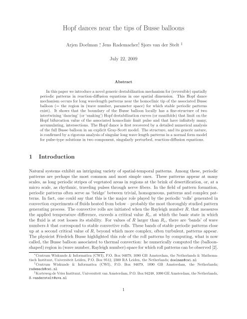
<strong>Hopf</strong> <strong>dances</strong> <strong>near</strong> <strong>the</strong> <strong>tips</strong> <strong>of</strong> <strong>Busse</strong> <strong>balloons</strong><br />
Arjen Doelman ∗ , Jens Rademacher † , Sjors van <strong>der</strong> Stelt ‡<br />
July 22, 2009<br />
Abstract<br />
In this paper we introduce a novel generic destabilization mechanism for (reversible) spatially<br />
periodic patterns in reaction-diffusion equations in one spatial dimension. This <strong>Hopf</strong> dance<br />
mechanism occurs for long wavelength patterns <strong>near</strong> <strong>the</strong> homoclinic tip <strong>of</strong> <strong>the</strong> associated <strong>Busse</strong><br />
balloon (= <strong>the</strong> region in (wave number, parameter space) for which stable periodic patterns<br />
exist). It shows that <strong>the</strong> boundary <strong>of</strong> <strong>the</strong> <strong>Busse</strong> balloon locally has a fine-structure <strong>of</strong> two<br />
intertwining ‘dancing’ (or ‘snaking’) <strong>Hopf</strong> destabilization curves (or manifolds) that limit on <strong>the</strong><br />
<strong>Hopf</strong> bifurcation value <strong>of</strong> <strong>the</strong> associated homoclinic limit pulse and that have infinitely many,<br />
accumulating, intersections. The <strong>Hopf</strong> dance is first recovered by a detailed numerical analysis<br />
<strong>of</strong> <strong>the</strong> full <strong>Busse</strong> balloon in an explicit Gray-Scott model. The structure, and its generic nature,<br />
is confirmed by a rigorous analysis <strong>of</strong> singular long wave length patterns in a normal form model<br />
for pulse-type solutions in two component, singularly perturbed, reaction-diffusion equations.<br />
1 Introduction<br />
Natural systems exhibit an intriguing variety <strong>of</strong> spatial-temporal patterns. Among <strong>the</strong>se, periodic<br />
patterns are perhaps <strong>the</strong> most common and most simple ones. These patterns appear at many<br />
scales, as long periodic stripes <strong>of</strong> vegetated areas in regions at <strong>the</strong> brink <strong>of</strong> desertification, or, at a<br />
micro scale, as rhythmic, traveling pulses through nerve fibers. In <strong>the</strong> field <strong>of</strong> pattern formation,<br />
periodic patterns <strong>of</strong>ten serve as ‘bridge’ between trivial, homogeneous, patterns and complex patterns.<br />
In fact, one could say that this is <strong>the</strong> major role played by <strong>the</strong> periodic ‘rolls’ generated in<br />
convection experiments <strong>of</strong> fluids heated from below – probably <strong>the</strong> most thoroughly studied pattern<br />
generating process. The convective rolls are initiated when <strong>the</strong> Rayleigh number R, that measures<br />
<strong>the</strong> applied temperature difference, exceeds a critical value R c , at which <strong>the</strong> basic state in which<br />
<strong>the</strong> fluid is at rest looses its stability. For values <strong>of</strong> R larger than R c , <strong>the</strong>re are ‘bands’ <strong>of</strong> wave<br />
numbers k that correspond to stable convective rolls. These bands <strong>of</strong> stable periodic patterns close<br />
up at a second critical value <strong>of</strong> R, beyond which more complex, <strong>of</strong>ten turbulent, patterns appear.<br />
The physicist Friedrich <strong>Busse</strong> highlighted this role <strong>of</strong> <strong>the</strong> roll patterns by computing, what is now<br />
called, <strong>the</strong> <strong>Busse</strong> balloon associated to <strong>the</strong>rmal convection: he numerically computed <strong>the</strong> (<strong>balloons</strong>haped)<br />
region in (wave number, Rayleigh number)-space for which roll patterns can be observed [2].<br />
∗ Centrum Wiskunde & Informatica (CWI), P.O. Box 94079, 1090 GB Amsterdam, <strong>the</strong> Ne<strong>the</strong>rlands & Ma<strong>the</strong>matisch<br />
Instituut, Universiteit Leiden, P.O. Box 9512, 2300 RA Leiden, <strong>the</strong> Ne<strong>the</strong>rlands; doelman@cwi.nl<br />
† Centrum Wiskunde & Informatica (CWI), P.O. Box 94079, 1090 GB Amsterdam, <strong>the</strong> Ne<strong>the</strong>rlands;<br />
rademach@cwi.nl<br />
‡ Korteweg-de Vries Instituut, Universiteit van Amsterdam, P.O. Box 94248, 1090 GE Amsterdam, <strong>the</strong> Ne<strong>the</strong>rlands,<br />
S.van<strong>der</strong>stelt@uva.nl<br />
1
The concept <strong>of</strong> ‘<strong>Busse</strong> balloon’ as a region in (wave number, parameter)-space in which stable<br />
periodic patterns exist, can <strong>of</strong> course also be defined in a more general setting (see §1.1). This<br />
paper is concerned with <strong>the</strong> study <strong>of</strong> generic properties <strong>of</strong> <strong>Busse</strong> <strong>balloons</strong> and/or <strong>the</strong> nature <strong>of</strong> <strong>the</strong><br />
boundary <strong>of</strong> <strong>Busse</strong> <strong>balloons</strong>. More specifically, this paper concerns <strong>the</strong> analysis <strong>of</strong> a novel generic<br />
mechanism that drives <strong>the</strong> destabilization <strong>of</strong> periodic patterns.<br />
A well-established example <strong>of</strong> such a mechanism comes from Ginzburg-Landau <strong>the</strong>ory, or equivalently,<br />
weakly nonli<strong>near</strong> stability <strong>the</strong>ory. This <strong>the</strong>ory shows that <strong>the</strong> evolution <strong>of</strong> patterns <strong>near</strong><br />
onset is (generically) governed by <strong>the</strong> (complex) Ginzburg-Landau equation. This equation exhibits<br />
bands <strong>of</strong> stable periodic patterns that are generically destabilized by <strong>the</strong> sideband (or Eckhaus, or<br />
Benjamin-Feir) instability mechanism. Moreover, <strong>the</strong> boundary <strong>of</strong> a <strong>Busse</strong> balloon <strong>near</strong> onset is<br />
generically given by a parabola – <strong>the</strong> Eckhaus parabola – <strong>of</strong> sideband destabilizations, see [1, 23]<br />
and <strong>the</strong> references <strong>the</strong>rein, and Remark 1.1. Ginzburg-Landau <strong>the</strong>ory is a general and very powerful<br />
<strong>the</strong>ory, however, it only applies to <strong>the</strong> asymptotically small part <strong>of</strong> a <strong>Busse</strong> balloon <strong>near</strong> onset. The<br />
main question that drove <strong>the</strong> research reported here is: ‘Is it possible to determine o<strong>the</strong>r destabilization<br />
mechanisms that describe generic structures <strong>of</strong> (<strong>the</strong> boundary <strong>of</strong>) a <strong>Busse</strong> balloon, that go<br />
beyond <strong>the</strong> sideband mechanism <strong>near</strong> onset?’.<br />
Of course, one can in general not hope to obtain a full analytical control over an entire <strong>Busse</strong><br />
balloon. As for <strong>the</strong> Ginzburg-Landau <strong>the</strong>ory one should only expect to be able to capture small,<br />
but essential, parts <strong>of</strong> <strong>the</strong> <strong>Busse</strong> balloon by analytical means (see however Remark 1.1). Moreover, it<br />
is at present too ambitious to propose to develop a <strong>the</strong>ory for ‘far-from-equilibrium-patterns’ that<br />
is as general as Ginzburg-Landau <strong>the</strong>ory. Based on recent developments in <strong>the</strong> (ma<strong>the</strong>matical)<br />
<strong>the</strong>ory, we never<strong>the</strong>less claim it is possible to consi<strong>der</strong> <strong>the</strong> above question in <strong>the</strong> setting <strong>of</strong> a wellspecified<br />
class <strong>of</strong> problems: <strong>the</strong> stability and destabilization <strong>of</strong> <strong>near</strong>ly localized, spatially periodic<br />
patterns in reaction-diffusion equations, see Figure 1. This class <strong>of</strong> problems is especially interesting,<br />
since <strong>the</strong>re are quite a number <strong>of</strong> results in <strong>the</strong> literature that indicate that <strong>the</strong>se (singular)<br />
long wavelength periodic multi-pulse/front/spike patterns appear as <strong>the</strong> ‘most stable’ – i.e <strong>the</strong> last<br />
periodic patterns to destabilize – spatially periodic patterns [8, 19, 20, 21, 24, 26, 29, 32, 43]. This<br />
is also confirmed by <strong>the</strong> <strong>Busse</strong> balloon for <strong>the</strong> Gray-Scott system (1.1) presented in Figure 2(a):<br />
for decreasing A, stable patterns appear at a Ginzburg-Landau/Turing bifurcation and eventually<br />
disappear at a ‘tip’ at which <strong>the</strong> wave number k approaches zero (i.e. at which <strong>the</strong> wavelength <strong>of</strong><br />
<strong>the</strong> patterns becomes large). Thus, <strong>the</strong>se singular patterns may indeed represent an essential (but<br />
small) part <strong>of</strong> <strong>the</strong> <strong>Busse</strong> balloon. Complementary to <strong>the</strong> small amplitude Ginzburg-Landau patterns<br />
that indicate <strong>the</strong> ‘bottom’ <strong>of</strong> <strong>the</strong> <strong>Busse</strong> balloon at which patterns appear, <strong>the</strong> <strong>near</strong>ly localized<br />
patterns may form <strong>the</strong> ‘tip’ <strong>of</strong> <strong>the</strong> <strong>Busse</strong> balloon at which <strong>the</strong> stable periodic patterns disappear.<br />
Therefore, we focus in this paper on <strong>the</strong> study <strong>of</strong> <strong>Busse</strong> <strong>balloons</strong> associated to periodic patterns in<br />
reaction-diffusion systems in one spatial dimension. In <strong>the</strong> numerical (first) part <strong>of</strong> <strong>the</strong> paper, we<br />
do consi<strong>der</strong> a ‘full’ <strong>Busse</strong> balloon, but only in <strong>the</strong> context <strong>of</strong> a very explicit, singularly perturbed<br />
two component model, <strong>the</strong> well-studied Gray-Scott equation,<br />
{<br />
Ut = U x x + A(1 − U) − UV 2<br />
V t = ε 4 V t t − BV + UV 2 , (1.1)<br />
in which A,B > 0 and ε > 0 are parameters (and 0 < ε ≪ 1 in <strong>the</strong> singularly perturbed setting). In<br />
<strong>the</strong> analytic part <strong>of</strong> <strong>the</strong> paper, we restrict ourselves to <strong>the</strong> <strong>near</strong>ly-localized tip <strong>of</strong> <strong>the</strong> <strong>Busse</strong> balloon,<br />
in <strong>the</strong> context <strong>of</strong> a certain (sub)class <strong>of</strong> problems that a priori includes <strong>the</strong> patterns consi<strong>der</strong>ed<br />
in <strong>the</strong> Gray-Scott model (see sections §1.2 and §3.5): <strong>the</strong> stability and destabilization <strong>of</strong> <strong>near</strong>ly<br />
2
1<br />
1<br />
0.8<br />
0.8<br />
U,V<br />
0.6<br />
U,V<br />
0.6<br />
0.4<br />
0.4<br />
0.2<br />
0.2<br />
0<br />
0<br />
0 20 40 60 80 100<br />
X<br />
0 20 40 60 80 100<br />
X<br />
Figure 1: Two typical stationary, <strong>near</strong>ly localized, reversible spatially periodic patterns with different<br />
wavelengths L/wave numbers k. These patterns coexist as stable solutions <strong>of</strong> <strong>the</strong> Gray-Scott<br />
model (1.1) with A = ε 4 = 0.01 and B = 0.060 [7].<br />
localized reversible patterns in singularly perturbed two component reaction-diffusion equations.<br />
The specific choice to restrict <strong>the</strong> analysis to singularly perturbed systems is motivated by <strong>the</strong><br />
state-<strong>of</strong>-<strong>the</strong>-art <strong>of</strong> <strong>the</strong> ma<strong>the</strong>matical <strong>the</strong>ory for <strong>the</strong> existence and stability <strong>of</strong> <strong>near</strong>ly localized periodic<br />
patterns. There is a well-developed qualitative ma<strong>the</strong>matical <strong>the</strong>ory for (one-dimensional) localized<br />
structures, such as (homoclinic) pulses/spikes and (heteroclinic) fronts, in reaction-diffusion<br />
equations – see [38] and <strong>the</strong> references <strong>the</strong>rein. By <strong>the</strong> methods developed in [16, 17, 39], it is possible<br />
to extend this <strong>the</strong>ory to <strong>near</strong>ly-localized spatially periodic patterns. However, at this point,<br />
<strong>the</strong> general <strong>the</strong>ory does not provide <strong>the</strong> amount <strong>of</strong> quantitative information necessary to study <strong>the</strong><br />
<strong>near</strong>ly homoclinic (k = 0) tip <strong>of</strong> <strong>Busse</strong> <strong>balloons</strong> in full detail. Such a more quantitative <strong>the</strong>ory has<br />
been developed in <strong>the</strong> context <strong>of</strong> singularly perturbed reaction-diffusion equations, both for <strong>the</strong><br />
localized patterns [8], as well as for <strong>the</strong> <strong>near</strong>ly-localized spatially periodic patterns [32]. We refer to<br />
section §6 for a discussion <strong>of</strong> <strong>the</strong> extension <strong>of</strong> our main results to non-singularly perturbed systems.<br />
The generic mechanism proposed here – <strong>the</strong> ‘<strong>Hopf</strong> dance <strong>near</strong> <strong>the</strong> tip <strong>of</strong> <strong>Busse</strong> <strong>balloons</strong>’ – is graphically<br />
presented in Figure 2. Figure 2(a) is <strong>the</strong> outcome <strong>of</strong> a comprehensive numerical study <strong>of</strong> <strong>the</strong><br />
stability and existence boundaries in (parameter,wave number)-space <strong>of</strong> spatially periodic patterns<br />
<strong>of</strong> <strong>the</strong> Gray-Scott model, by means <strong>of</strong> continuation techniques (see especially [34]). Although <strong>the</strong><br />
Gray-Scott system is one <strong>of</strong> <strong>the</strong> most thoroughly studied reaction-diffusion systems in <strong>the</strong> recent<br />
literature, see e.g. [7, 9, 11, 20, 21, 24, 25, 26, 27, 28, 31, 33, 37, 44], we are not aware <strong>of</strong> a comparable<br />
comprehensive (numerical) study <strong>of</strong> periodic patterns in <strong>the</strong> Gray-Scott model (a rough<br />
approximation <strong>of</strong> this <strong>Busse</strong> balloon, obtained by direct simulation <strong>the</strong> Gray-Scott model, has been<br />
presented in [24]; in [42] <strong>the</strong> same continuation approach has been used to study <strong>the</strong> stability <strong>of</strong><br />
periodic patterns in lambda-omega systems). The ‘<strong>Hopf</strong> dance’ is performed by two intertwined<br />
snaking curves <strong>of</strong> <strong>Hopf</strong> instabilities, denoted by H ±1 in Figure 2, that terminate in <strong>the</strong> limit k = 0<br />
at <strong>the</strong> <strong>Hopf</strong> bifurcation <strong>of</strong> <strong>the</strong> limiting homoclinic pulse. Figure 2(b) gives a schematic sketch <strong>of</strong><br />
<strong>the</strong> <strong>Hopf</strong> dance destabilization mechanism. The curve H +1 , represents a <strong>Hopf</strong> destabilization in<br />
which all extrema <strong>of</strong> <strong>the</strong> pattern starts to oscillate exactly in phase at <strong>the</strong> bifurcation; at H −1 <strong>the</strong><br />
3
17.5<br />
15.0<br />
equilibrium<br />
k<br />
12.5<br />
10.0<br />
7.5<br />
5.0<br />
sn<br />
1<br />
H +1<br />
sideband<br />
<strong>Busse</strong> balloon<br />
1.00<br />
2.5<br />
0.75 1 H<br />
0.50<br />
+1<br />
0.25<br />
equilibrium H<br />
0.00<br />
−1<br />
0.000 0.010 0.020 0.030 0.040 0.050<br />
0.0<br />
0.00 0.25 0.50 0.75 1.00 1.25 1.50 1.75 2.00<br />
sn<br />
A<br />
2<br />
2.00<br />
1.75<br />
1.50<br />
1.25<br />
sideband<br />
sn<br />
k<br />
H −1<br />
H +1<br />
<strong>Busse</strong>−balloon<br />
µ H µ<br />
(a)<br />
(b)<br />
Figure 2: (a) A <strong>Busse</strong> balloon associated to <strong>the</strong> Gray-Scott equation, (1.1) with B = 0.26 and<br />
ε 4 = 0.001, embedded in <strong>the</strong> associated existence balloon, i.e. <strong>the</strong> region in (parameter,wave<br />
number)-space in which spatially periodic patterns exist (but are not necessarily stable). For<br />
decreasing A, <strong>the</strong> <strong>Busse</strong> balloon is initiated by a Turing/Ginzburg-Landau bifurcation; it ends at<br />
a ‘homoclinic tip’ at A <strong>of</strong> <strong>the</strong> or<strong>der</strong> <strong>of</strong> ε 4 . The boundary segments are labeled according to <strong>the</strong>ir<br />
type: for existence <strong>the</strong>se are curves <strong>of</strong> folds (sn 1 , sn 2 ) and <strong>of</strong> vanishing amplitude at equilibria;<br />
for stability <strong>the</strong>se are curves <strong>of</strong> <strong>Hopf</strong> instabilities, sideband instabilities and also folds – <strong>the</strong> exact<br />
meaning and interpretation <strong>of</strong> <strong>the</strong>se labels are discussed in detail in section §3. Bullets mark corners<br />
(co-dimension 2 points). The inset enlarges <strong>the</strong> rectangular region <strong>near</strong> <strong>the</strong> homoclinic (k = 0) limit<br />
at which <strong>the</strong> <strong>Hopf</strong> dance <strong>of</strong> <strong>the</strong> curves H ±1 occurs. Note that only <strong>the</strong> first three intersections <strong>of</strong><br />
<strong>the</strong> curves H ±1 have been plotted. (b) A schematic sketch <strong>of</strong> <strong>the</strong> <strong>Hopf</strong> dance at <strong>the</strong> homoclinic tip<br />
<strong>of</strong> a <strong>Busse</strong> balloon; µ is a parameter and µ H indicates <strong>the</strong> <strong>Hopf</strong> bifurcation value associated to <strong>the</strong><br />
homoclinic pulse pattern that appears as k ↓ 0.<br />
maximums (or minimums) <strong>of</strong> <strong>the</strong> patterns that are one period away from each o<strong>the</strong>r begin to oscillate<br />
exactly out <strong>of</strong> phase. The <strong>Hopf</strong> dance gives <strong>the</strong> boundary <strong>of</strong> <strong>the</strong> <strong>Busse</strong> balloon a fine-structure<br />
<strong>of</strong> alternating pieces <strong>of</strong> <strong>the</strong> curves H +1 and H −1 , representing different types <strong>of</strong> destabilizations,<br />
separated by an infinite sequence <strong>of</strong> corners, or co-dimension 2 points.<br />
The H ±1 <strong>Hopf</strong> instabilities stem from <strong>the</strong> intersections with <strong>the</strong> imaginary axis <strong>of</strong> <strong>the</strong> endpoints<br />
<strong>of</strong> a bounded curve <strong>of</strong> <strong>the</strong> spectrum associated to <strong>the</strong> li<strong>near</strong>ized stability <strong>of</strong> <strong>the</strong> periodic pattern<br />
(see section §2). To leading or<strong>der</strong>, this spectral curve is a straight line segment that, as a function<br />
<strong>of</strong> decreasing wave number k, rotates around its center while shrinking exponentially in length.<br />
At second or<strong>der</strong>, <strong>the</strong> spectral curve is bended, and it is striking to note that its overall curvature<br />
oscillates with twice <strong>the</strong> frequency <strong>of</strong> <strong>the</strong> rotation, so that <strong>the</strong> most unstable point <strong>of</strong> <strong>the</strong> spectral<br />
curve cannot be an interior point, but must always be one <strong>of</strong> <strong>the</strong> two H ±1 endpoints. In this paper,<br />
we refer to this oscillation as <strong>the</strong> ‘belly dance’.<br />
A priori, <strong>the</strong> <strong>Hopf</strong> (and belly) dance performed by <strong>the</strong> (spectrum associated to <strong>the</strong>) periodic patterns<br />
in <strong>the</strong> Gray-Scott model may seem like very special, and thus non-generic, behavior. However,<br />
this is not <strong>the</strong> case. In <strong>the</strong> second part <strong>of</strong> this paper, §4–§5, we prove that both <strong>the</strong> <strong>Hopf</strong> and <strong>the</strong><br />
4
elly <strong>dances</strong> occur in a class <strong>of</strong> two component, singularly perturbed reaction-diffusion systems<br />
that includes <strong>the</strong> generalized Gierer-Meinhardt model [8]. Based on <strong>the</strong> Evans function analysis<br />
<strong>of</strong> [32], we give explicit formulas for <strong>the</strong> leading and next or<strong>der</strong> geometry <strong>of</strong> <strong>the</strong> spectral curves<br />
associated to <strong>the</strong> stability <strong>of</strong> <strong>the</strong> <strong>near</strong>ly localized spatially periodic patterns in this class <strong>of</strong> systems.<br />
In particular, our formulas give explicit expressions (in terms <strong>of</strong> exponentially small quantities in<br />
ε) for <strong>the</strong> local (fine-)structure <strong>of</strong> <strong>the</strong> boundary <strong>of</strong> <strong>the</strong> <strong>Busse</strong> balloon. Moreover, we identify <strong>the</strong><br />
quantity that determines whe<strong>the</strong>r <strong>the</strong> limiting homoclinic k = 0 pulse is <strong>the</strong> last periodic pattern<br />
to become unstable as <strong>the</strong> parameter varies (called Ni’s conjecture [29], see Remark 5.3). Similarly,<br />
we identify <strong>the</strong> quantity that determines <strong>the</strong> orientation <strong>of</strong> <strong>the</strong> belly dance, that is, whe<strong>the</strong>r <strong>the</strong><br />
H ±1 endpoints <strong>of</strong> <strong>the</strong> spectral curves are always <strong>the</strong> most unstable or not. In <strong>the</strong> latter case, <strong>the</strong><br />
actual stability boundary will be a smoo<strong>the</strong>d out version <strong>of</strong> that obtained from consi<strong>der</strong>ing <strong>the</strong><br />
endpoints alone, see Figure 10 and section §6.<br />
We conclude this paper by a discussion <strong>of</strong> <strong>the</strong> robustness <strong>of</strong> <strong>the</strong> <strong>Hopf</strong> dance destabilization mechanism<br />
within larger classes <strong>of</strong> systems (section §6).<br />
Remark 1.1 An important class <strong>of</strong> equations with a rich, and relatively easy to study, class <strong>of</strong><br />
periodic patterns (or wave trains) is <strong>the</strong> widely studied complex Ginzburg-Landau equation. In<br />
<strong>the</strong> most simple case, <strong>the</strong> real Ginzburg-Landau equation, <strong>the</strong> boundary <strong>of</strong> <strong>the</strong> <strong>Busse</strong> balloon<br />
is in its entirety given by <strong>the</strong> (unbounded) Eckhaus parabola <strong>of</strong> sideband instabilities. For <strong>the</strong><br />
general (complex) cubic Ginzburg-Landau equation, <strong>the</strong> <strong>Busse</strong> balloon may be non-existent, or its<br />
boundary may consist <strong>of</strong> certain <strong>Hopf</strong> bifurcations [22]. The structure <strong>of</strong> <strong>the</strong> <strong>Busse</strong> balloon becomes<br />
less simple, and for instance includes co-dimension 2 corners, for (extended) cubic-quintic Ginzburg-<br />
Landau equations that occur <strong>near</strong> <strong>the</strong> transition <strong>of</strong> super- to subcritical bifurcations [6, 14, 40, 41].<br />
In fact, <strong>the</strong> analysis in [14] indicates that <strong>the</strong>re may even be bounded <strong>Busse</strong> <strong>balloons</strong> in this case.<br />
Remark 1.2 Some aspects <strong>of</strong> <strong>the</strong> <strong>Hopf</strong> dance destabilization mechanism were already found analytically<br />
in [32] for <strong>the</strong> special case <strong>of</strong> <strong>the</strong> classical Gierer-Meinhardt model. However, it was not<br />
yet recognized in [32] as a generic phenomenon, and not analyzed in detail.<br />
1.1 The setting<br />
In <strong>the</strong>ir most general form, two component reaction-diffusion equations in one spatial dimension<br />
are given by, {<br />
Ut = U xx + F(U,V ; ⃗µ)<br />
V t = D 2 (1.2)<br />
V xx + G(U,V ;⃗µ)<br />
The reaction is described by <strong>the</strong> vector fields F,G : R 2 → R 2 that depend on <strong>the</strong> parameter(s)<br />
⃗µ ∈ R m (m ≥ 1) in <strong>the</strong> problem. The system is consi<strong>der</strong>ed on <strong>the</strong> unbounded real line, i.e. x ∈ R,<br />
and x is scaled such that <strong>the</strong> diffusion coefficient associated to U is 1; V diffuses with coefficient<br />
D 2 > 0.<br />
The stationary problem associated to (1.2) consists <strong>of</strong> two purely second or<strong>der</strong> ordinary differential<br />
equations in <strong>the</strong> time-like space variable x. Such equations always possess a reversible symmetry<br />
induced by spatial reflection x → −x. Solutions that are reflection symmetric in x are called<br />
reversible, which is <strong>the</strong> case for all solutions that are relevant for our purposes. Reflection symmetric<br />
periodic patterns, or standing wave trains, <strong>of</strong> (1.1) are reversible periodic orbits and typically<br />
persist as periodic orbits un<strong>der</strong> perturbation with an adjusted period L (or wave number k), e.g.,<br />
[13, 35]. Hence, we can expect open regions <strong>of</strong> existence in <strong>the</strong> (⃗µ,k)-parameter space.<br />
5
Let (U p (x;k),V p (x;k)) be such a family <strong>of</strong> stationary spatially periodic patterns with associated<br />
periodic solutions γ p (x;k) <strong>of</strong> <strong>the</strong> 4-dimensional (spatial) dynamical system for stationary solutions<br />
<strong>of</strong> (1.2). Existence regions <strong>the</strong>n come as (maximal) connected regions I e (⃗µ) ⊂ R in k for which<br />
(U p (x;k),V p (x;k)) exist. Note that for a given ⃗µ, I e (⃗µ) may only be one <strong>of</strong> several disjoint existence<br />
regions. The physically most relevant patterns are <strong>the</strong> solutions <strong>of</strong> (1.2) that are dynamically<br />
stable. In this paper we are only concerned with spectral stability. We define σ = σ(U p ,V p ) as<br />
<strong>the</strong> spectrum associated to <strong>the</strong> li<strong>near</strong>ization about a pattern (U p (x;k),V p (x;k)) (1.2) and call a<br />
pattern spectrally stable if σ ∩ {Re(λ) ≥ 0} = {0}, and if <strong>the</strong> curve <strong>of</strong> σ through <strong>the</strong> origin has<br />
quadratic tangency, see e.g, [35]. Stable periodic patterns form a subset <strong>of</strong> I e (⃗µ). Let I s (⃗µ) ⊂ I e (⃗µ)<br />
be a connected component <strong>of</strong> this subset in <strong>the</strong> sense that (U p (x;k),V p (x;k)) destabilizes as k approaches<br />
<strong>the</strong> boundary <strong>of</strong> I s (⃗µ). A <strong>Busse</strong> balloon B B <strong>of</strong> (1.2) is defined as a connected component<br />
<strong>of</strong> <strong>the</strong> (⃗µ,k)-parameters <strong>of</strong> stable periodic patterns, that is,<br />
B B = ⋃<br />
µ∈R M I s (µ) ⊂ R M+1 , (1.3)<br />
see also Remark 1.3. For practical reasons, one <strong>of</strong>ten fixes (m − 1)-components <strong>of</strong> ⃗µ and only plots<br />
a two-dimensional cross-section <strong>of</strong> B B in (µ j ,k)-space – see Figure 2.<br />
The reversible symmetry has consequences for <strong>the</strong> (stability) boundary <strong>of</strong> <strong>the</strong> <strong>Busse</strong> balloon. According<br />
to [36], <strong>the</strong> following types <strong>of</strong> instabilities with respect to destabilizing modes e i(αt+ηx) can<br />
occur along curves <strong>of</strong> <strong>the</strong> boundary:<br />
‘sideband’ tangency <strong>of</strong> <strong>the</strong> curve <strong>of</strong> σ at <strong>the</strong> origin changes sign<br />
(also called Benjamin-Feir or Eckhaus instability)<br />
‘<strong>Hopf</strong>’ <strong>the</strong>re exists α ≠ 0, such that {iα,0} = σ ∩ {Re(λ) ≥ 0}<br />
‘Turing’ as <strong>Hopf</strong>, but with α = 0,<br />
‘Period doubling’ as Turing, but with η = k/2,<br />
‘Pure <strong>Hopf</strong>’ as <strong>Hopf</strong> with α ≠ 0, η = 0,<br />
‘Fold’ <strong>the</strong> pattern un<strong>der</strong>goes a saddle-node bifurcation.<br />
Inspired by <strong>the</strong> <strong>Hopf</strong> dance observed in <strong>the</strong> Gray-Scott model, we focus in <strong>the</strong> analytic part <strong>of</strong><br />
this paper on <strong>the</strong> ‘normal form model’ for large amplitude pulse patterns to singularly perturbed<br />
equations given by { ε 2 U t = U xx − ε 2 µU + U α 1<br />
V β 1<br />
V t = ε 2 V xx − V + U α 2<br />
V β 2<br />
(1.4)<br />
,<br />
in which 0 < ε ≪ 1. This model is known as <strong>the</strong> generalized Gierer-Meinhardt equation [8, 18, 19,<br />
29, 43, 45]; U(x,t),V (x,t) are scaled versions <strong>of</strong> <strong>the</strong>ir counterparts in (1.2) and are by construction<br />
O(1) w.r.t. ε. This equation was originally <strong>der</strong>ived as leading or<strong>der</strong> normal form model for large<br />
amplitude pulse patterns to singularly perturbed two component reaction-diffusion equations in [8].<br />
It is <strong>der</strong>ived from equations <strong>of</strong> <strong>the</strong> type (1.2) by imposing a couple <strong>of</strong> assumptions:<br />
(A-i) <strong>the</strong> system has a stable ‘background state’ (U(x,t),V (x,t)) ≡ (0,0);<br />
(A-ii) <strong>the</strong> equations decouple at <strong>the</strong> li<strong>near</strong> level (i.e. as ‖(U,V )‖ becomes small);<br />
(A-iii) <strong>the</strong> nonli<strong>near</strong>ities grow algebraically and are ‘separable’ in a sense explained in §1.2.<br />
We refer to section §1.2 for a sketch <strong>the</strong> <strong>der</strong>ivation <strong>of</strong> (1.4) and <strong>the</strong> conditions on its parameters.<br />
As for <strong>the</strong> Gray-Scott model, <strong>the</strong>re are many indications in <strong>the</strong> literature that tip <strong>of</strong> <strong>the</strong><br />
<strong>Busse</strong> balloon associated to (1.4), i.e. <strong>the</strong> last region in which stable periodic patterns exist, is also<br />
formed by <strong>near</strong>ly homoclinic, <strong>near</strong>ly localized, spatially periodic patterns [8, 19, 29, 32, 43]. More<br />
6
specifically, <strong>the</strong> limiting homoclinic k = 0 pattern generally appears as ‘<strong>the</strong> last pattern to become<br />
unstable’ – see §5 and particularly Remark 5.3 on Ni’s conjecture. In section §4, (part <strong>of</strong>) <strong>the</strong><br />
existing literature on <strong>the</strong> existence and stability <strong>of</strong> stationary singular spatially periodic patterns<br />
to (1.4) is summarized.<br />
Remark 1.3 Reaction-diffusion equations naturally also exhibit traveling spatially periodic patterns,<br />
or wave trains, i.e. non-stationary solutions that are periodic in space and in time. For <strong>the</strong>se<br />
patterns, one can also define <strong>the</strong> concept <strong>of</strong> a <strong>Busse</strong> balloon (in a completely equivalent fashion).<br />
However, in this paper we only consi<strong>der</strong> stationary periodic patterns.<br />
1.2 The normal form model<br />
In this section we give a brief <strong>der</strong>ivation <strong>of</strong> (1.4) as normal form model for large amplitude pulses in<br />
<strong>the</strong> general class <strong>of</strong> singularly perturbed (two component) reaction-diffusion models (1.2). First, we<br />
bring <strong>the</strong> equation into a singularly perturbed form that satisfies <strong>the</strong> first two assumptions ((A-i)<br />
and (A-ii),<br />
{<br />
Ut = U xx − µU + H 1 (U,V ;ε, ⃗µ)<br />
V t = ε 4 (1.5)<br />
V xx − V + H 2 (U,V ;ε, ⃗µ),<br />
where H j = O(2). Note that <strong>the</strong> parameter µ controls <strong>the</strong> (relative) decay rates <strong>of</strong> U and V (i.e.<br />
µ > 0). Singular equations <strong>of</strong> this type generally exhibit localized patterns that are singular in<br />
various ways: (E-i) <strong>the</strong> ‘fast’ V -components are spatially localized in regions in which <strong>the</strong> ‘slow’<br />
component U remains at leading or<strong>der</strong> constant; (E-ii) <strong>the</strong> U-components vary slowly in regions<br />
in which V is exponentially small; (E-iii) <strong>the</strong> amplitude <strong>of</strong> both U- and V -components scale with<br />
a negative power <strong>of</strong> ε – i.e. <strong>the</strong>y are asymptotically large. Therefore, it is natural to scale out <strong>the</strong><br />
asymptotic magnitudes <strong>of</strong> U and V ,<br />
Ũ(x,t) = ε r U(x,t),r ≥ 0, Ṽ (x,t) = ε s V (x,t),s ≥ 0,<br />
so that Ũ(x,t) and Ṽ (x,t) are O(1) w.r.t. ε; <strong>the</strong> magnitudes r and s are a priori unknown. The<br />
following assumption on <strong>the</strong> asymptotic behavior <strong>of</strong> <strong>the</strong> nonli<strong>near</strong>ities H 1,2 (U,V ), which is <strong>the</strong><br />
technical version <strong>of</strong> assumption (A-iii), is crucial to <strong>the</strong> <strong>der</strong>ivation <strong>of</strong> (1.4),<br />
H i (U,V ) = H i (Ũ<br />
ε r , Ṽ<br />
[ ]<br />
ε s) = Ũα i<br />
Ṽ β i<br />
ε −(rα i+sβ i )<br />
h i + ˆε ˜H(Ũ,Ṽ ;ε) , (1.6)<br />
in which ˆε is some positive power <strong>of</strong> ε and ˜H i = O(1) w.r.t. ε. Hence, it is assumed that <strong>the</strong> growth<br />
<strong>of</strong> nonli<strong>near</strong> terms H i (U,V ) for U,V large is dominated by <strong>the</strong> algebraic expression U α i<br />
V β i<br />
. Note<br />
that this part <strong>of</strong> assumption (A-iii) is quite natural, as are assumptions (A-i) and (A-ii) – see<br />
Remark 1.4. However, <strong>the</strong>re is an additional part to assumption (A-iii) that is more restrictive:<br />
<strong>the</strong> asymptotic decomposition (1.6) is also assumed to be separable, in <strong>the</strong> sense that <strong>the</strong> leading<br />
or<strong>der</strong> terms (for U,V large) can be factored out <strong>of</strong> H i (U,V ). Note that this assumption for instance<br />
implies that H i → 0 as V i → 0 (1.8), i.e. it implies that <strong>the</strong> leading or<strong>der</strong> behavior for large solutions<br />
also dominates as <strong>the</strong>se solutions are no longer large. See §6 and Remark 1.4 for a discussion <strong>of</strong><br />
this issue and its relation to <strong>the</strong> (conjectured) generiticity <strong>of</strong> <strong>the</strong> <strong>Hopf</strong> dance. The magnitudes r<br />
and s <strong>of</strong> U and V can now be determined in terms <strong>of</strong> α 1 ,α 2 ,β 1 ,β 2 by <strong>the</strong> assumption that (large,<br />
singular) pulse type patterns can indeed exist as solutions <strong>of</strong> (1.5),<br />
r = β 2 − 1<br />
d<br />
> 0, s = − α 2<br />
d<br />
> 0, with d<br />
def<br />
= (α 1 − 1)(β 2 − 1) − α 2 β 1 > 0, (1.7)<br />
7
see [8]. This analysis also yields that h j > 0, for j = 1,2, and that <strong>the</strong> parameter(s) ⃗µ =<br />
(µ,α 1 ,α 2 ,β 1 ,β 2 ) in (1.4) must satisfy <strong>the</strong> following conditions,<br />
µ > 0, d > 0, α 2 < 0, β 1 > 1, β 2 > 1. (1.8)<br />
By introducing <strong>the</strong> spatial scale ˜x = x/ε and neglecting all tildes, equation (1.5) can now at leading<br />
or<strong>der</strong> be brought into <strong>the</strong> ‘normal form’ (1.4).<br />
Remark 1.4 A more general model that satisfies (A-i) and (A-ii) and that generalizes (A-iii) to<br />
non-separable nonli<strong>near</strong>ities is,<br />
{ ε 2 U t = U xx − ε 2 [µU − F 1 (U;ε)] + F 2 (U,V ;ε),<br />
V t = ε 2 (1.9)<br />
V xx − V + G(U,V ;ε).<br />
Note that especially <strong>the</strong> fact that <strong>the</strong>re is a spatial nonli<strong>near</strong>ity F 1 (U;ε) ≠ 0 distinguishes this<br />
model from <strong>the</strong> Gray-Scott/Gierer-Meinhardt types models in <strong>the</strong> literature [5]. We will come back<br />
to this generalized model in <strong>the</strong> discussion <strong>of</strong> <strong>the</strong> (non-)generic effect <strong>of</strong> <strong>the</strong> ‘belly dance’ in section<br />
§6.<br />
2 Preliminaries I: The stability <strong>of</strong> periodic patterns<br />
In this section, we sketch several aspects <strong>of</strong> <strong>the</strong> literature on <strong>the</strong> stability <strong>of</strong> periodic patterns<br />
in reaction-diffusion equations. The presentation is largely based on [16, 17, 32, 34, 35, 39]. For<br />
simplicity, we restrict ourselves to <strong>the</strong> two components setting <strong>of</strong> (1.2). However, <strong>the</strong> ideas presented<br />
here can be readily extended to N-component systems. Moreover, (1.2) includes all o<strong>the</strong>r, more<br />
specific, models consi<strong>der</strong>ed in this paper.<br />
2.1 The structure <strong>of</strong> <strong>the</strong> spectrum<br />
The spectral stability problem associated to a stationary, spatially periodic solution (U p (x;k),V p (x;k))<br />
<strong>of</strong> (1.2) with respect to perturbations (for instance) in BC unif (R, R 2 ), i.e. <strong>the</strong> space <strong>of</strong> bounded<br />
and uniformly continuous functions, is obtained by substitution <strong>of</strong><br />
U(x,t) = U p (x;k) + u(x)e λt , V (x,t) = V p (x;k) + v(x)e λt ,<br />
into (1.4), followed by li<strong>near</strong>ization. This yields <strong>the</strong> system,<br />
{ λu = uxx + ∂ U F(U p (x),V p (x))u + ∂ V F(U p (x),V p (x))v<br />
λv = D 2 v xx + ∂ U G(U p (x),V p (x))u + ∂ V G(U p (x),V p (x))v<br />
(2.1)<br />
Since x ∈ R, (2.1) can be written in <strong>the</strong> form <strong>of</strong> a 4-dimensional (li<strong>near</strong>) system,<br />
˙φ(ξ) = A p (ξ;λ,L,ε)φ(ξ), (2.2)<br />
where φ = (u,p = Du ξ ,v,q = v ξ ) t in <strong>the</strong> scaled spatial variable ξ = x/D and <strong>the</strong> dot denotes<br />
differentiation with respect to ξ. Note that ξ is introduced in anticipation <strong>of</strong> <strong>the</strong> singularly perturbed<br />
setting in which ξ represents <strong>the</strong> ‘fast’ spatial scale. For <strong>the</strong> same reason, we introduce<br />
8
L as half <strong>of</strong> <strong>the</strong> wavelength <strong>of</strong> <strong>the</strong> periodic pattern (U p ,V p ), i.e., with a slight abuse <strong>of</strong> notation,<br />
(U p (x;k),V p (x;k)) = (U p (ξ;L),V p (ξ;L)) with L = π/kD. Therefore, <strong>the</strong> periodic matrix<br />
A p (ξ;λ,k) in (2.2) is given by,<br />
A p (ξ;λ,L) =<br />
⎛<br />
⎜<br />
⎝<br />
0 D 0 0<br />
D(λ − ∂ U F(U p (ξ;L),V p (ξ;L))) 0 −D∂ V F(U p (ξ;L),V p (ξ;L)) 0<br />
0 0 0 1<br />
−∂ U G(U p (ξ;L),V p (ξ;L)) 0 (λ − ∂ V G(U p (ξ;L),V p (ξ;L))) 0<br />
⎞<br />
⎟<br />
⎠ . (2.3)<br />
Since A p (ξ;λ,L) is 2L periodic, solutions to (2.2) can (by Floquet <strong>the</strong>ory) be assumed to be <strong>of</strong> <strong>the</strong><br />
form<br />
φ(ξ) = ψ(ξ)e cξ for some c ∈ C and ψ(ξ) 2L−periodic.<br />
However, <strong>the</strong> perturbations φ(ξ;λ) must be in BC(R, C 4 ), so that c = i˜c ∈ iR. Hence,<br />
φ(ξ + 2L;λ) = γ φ(ξ;λ) for a γ ∈ S 1 , (2.4)<br />
since γ = e 2i˜cL ∈ C with |γ| = 1. Note that if φ(ξ;λ) satisfies condition (2.4) in one particular<br />
point ξ, it satisfies (2.4) everywhere. Since bounded solutions <strong>of</strong> (2.2) can be decomposed into a<br />
combination <strong>of</strong> functions φ(ξ;λ) that satisfy (2.4) for some γ ∈ S 1 , it follows that <strong>the</strong> spectrum<br />
σ((U p ,V p )) <strong>of</strong> <strong>the</strong> stability problem associated to <strong>the</strong> periodic pattern (U p (ξ;L),V p (ξ;L)) entirely<br />
consists <strong>of</strong> γ-eigenvalues [16], i.e. λ(γ) ∈ C such that <strong>the</strong>re is a solution φ(ξ) <strong>of</strong> (2.2) that satisfies<br />
(2.4) for some γ ∈ S 1 . Thus, by varying γ over S 1 , we may conclude that σ((U p ,V p )) is <strong>the</strong> union<br />
<strong>of</strong> – a priori countably many – bounded curves Λ(L; ⃗µ) with<br />
Λ(L; ⃗µ) = {λ ∈ C : λ(γ) is a γ−eigenvalue,γ ∈ S 1 } (2.5)<br />
(see [16, 34, 39]). In general, <strong>the</strong>se curves can ei<strong>the</strong>r be a smooth image <strong>of</strong> S 1 or have a more degenerate<br />
structure. In particular, <strong>the</strong>y <strong>of</strong>ten form closed loops that are isolated connected components<br />
<strong>of</strong> <strong>the</strong> spectrum.<br />
2.2 Reversibility: <strong>the</strong> collapse <strong>of</strong> Λ(L; ⃗µ)<br />
Due to <strong>the</strong> reversibility symmetry in both <strong>the</strong> equation (1.2) and <strong>the</strong> patterns (U p (ξ;L),V p (ξ;L)),<br />
<strong>the</strong> spectral loops Λ(L; ⃗µ) (2.5) collapse to branches with well-defined endpoints ∂ ± Λ(L; ⃗µ). To<br />
see this, we need to be more explicit about nature <strong>of</strong> <strong>the</strong>se symmetries. First, we may define<br />
ξ = 0 as a reflection point for <strong>the</strong> pattern (U p (ξ;L),V p (ξ;L)), i.e. we may assume that<br />
(U p (−ξ;L),V p (−ξ;L)) = (U p (ξ;L),V p (ξ;L)) for all ξ. Note that,<br />
(U p (L + ξ),V p (L + ξ;L)) = (U p (ξ − L),V p (ξ − L)) = (U p (L − ξ),V p (L − ξ))<br />
by <strong>the</strong> 2L-periodicity <strong>of</strong> (U p (ξ;L),V p (ξ;L)). Hence, (U p (ξ;L),V p (ξ;L)), and thus A p (ξ;L) (2.3), is<br />
reflection symmetric with respect to all points ξ = kL, k ∈ Z. Thus, system (2.2) is also reversible,<br />
i.e. if φ(ξ) is a solution, <strong>the</strong>n so is ˆφ(ξ), with<br />
ˆφ(ξ) = Rφ(−ξ) = (u(−ξ), −p(−ξ),v(−ξ), −q(−ξ)).<br />
Now, if λ is a γ-eigenvalue, and φ(ξ) its associated γ-eigenfunction, <strong>the</strong>n (by (2.4)),<br />
ˆφ(ξ + 2L) = Rφ(−ξ − 2L) = 1 Rφ(−ξ) = γ ˆφ(ξ),<br />
γ<br />
9
since γ ∈ S 1 . In o<strong>the</strong>r words, ˆφ(ξ) is a γ-eigenfunction (2.4), which implies that λ is both a γ- and<br />
a γ-eigenvalue. Hence, as γ is varied over S 1 , every point λ(γ) ∈ Λ(L; ⃗µ) is visited twice, except for<br />
<strong>the</strong> points λ(±1) since γ = γ for γ = ±1: <strong>the</strong> loop Λ(L; ⃗µ) collapses to a branch with endpoints<br />
∂ ± Λ(L; ⃗µ) = γ(±1)<br />
If a branch Λ(L; ⃗µ) crosses through <strong>the</strong> imaginary axis as a function <strong>of</strong> ⃗µ, it is very likely that<br />
one <strong>of</strong> <strong>the</strong> endpoints ∂ ± Λ(L; ⃗µ) is <strong>the</strong> first point <strong>of</strong> Λ(L; ⃗µ) to make contact with <strong>the</strong> imaginary<br />
axis. Indeed, if this occurs, it is robust un<strong>der</strong> perturbations. However, note that this is not necessary:<br />
Λ(L; ⃗µ) ⊂ C is in general curved, so Λ(L; ⃗µ) may be tangent to <strong>the</strong> imaginary axis at its<br />
point λ(γ) <strong>of</strong> first contact, i.e. λ(γ) may certainly be an interior point with γ ≠ ±1. Even when<br />
Λ(L; ⃗µ) ⊂ R, <strong>the</strong> possibility that Λ(L; ⃗µ) is folded cannot be excluded, so that <strong>the</strong> first point <strong>of</strong><br />
contact <strong>of</strong> Λ(L; ⃗µ) with <strong>the</strong> imaginary axis is not necessarily an endpoint ∂ ± Λ(L; ⃗µ), but possibly an<br />
interior point at <strong>the</strong> fold. Never<strong>the</strong>less, it can be expected that <strong>the</strong> ±1-eigenvalues do play a dominant<br />
role in <strong>the</strong> stability and bifurcation analysis <strong>of</strong> reversible periodic patterns (U p (ξ;L),V p (ξ;L)).<br />
And thus, <strong>the</strong> bifurcations associated to <strong>the</strong>se eigenvalues can be expected to turn up abundantly<br />
in <strong>the</strong> study <strong>of</strong> <strong>Busse</strong> <strong>balloons</strong> B B .<br />
We <strong>the</strong>refore define µ ± as <strong>the</strong> following critical value <strong>of</strong> µ, where µ represents one <strong>of</strong> <strong>the</strong> m components<br />
<strong>of</strong> ⃗µ: Re[σ(U p ,V p )] < 0 for µ < µ ± , Re[σ(U p ,V p )] = 0 only for a ∂ ± Λ(L; ⃗µ) ∈ σ(U p ,V p )<br />
at µ = µ ± and Re[∂ ± Λ(L; ⃗µ) > 0 for µ > µ ± (this situation occurs in <strong>the</strong> Gray-Scott system,<br />
§3, and in <strong>the</strong> normal form model (1.4), §5). A priori, we need to distinguish between two cases:<br />
Im[∂ ± Λ(L;µ = µ ± )] = 0 and Im[∂ ± Λ(L;µ = µ ± )] ≠ 0. However, in this paper we focus on <strong>the</strong><br />
latter case. We refer to [32] for an example at which ∂ − Λ(L;µ j = µ ± ) ∈ R initiates a saddle node<br />
bifurcation.<br />
The +1-eigenfunction φ(ξ;λ(+1)) associated to ∂ + Λ(L;µ = µ + ) is 2L-periodic (by (2.4)). Since<br />
∂ + Λ(L;µ = µ + ) induces a <strong>Hopf</strong> instability if Im[∂ + Λ(L;µ = µ + )] ≠ 0 [35], this means that <strong>the</strong><br />
destabilization at µ = µ + initiates an oscillation at which all extrema <strong>of</strong> <strong>the</strong> pattern (U p (ξ;L),V p (ξ;L))<br />
move in phase. Note that description is only based on li<strong>near</strong> data, without fur<strong>the</strong>r analysis it is not<br />
possible to extract information about <strong>the</strong> nonli<strong>near</strong>, long-time, behavior beyond <strong>the</strong> bifurcation.<br />
Never<strong>the</strong>less, this li<strong>near</strong> prediction agrees with <strong>the</strong> (subcritical) <strong>Hopf</strong> bifurcation destabilization<br />
<strong>of</strong> +1-type most commonly encountered in simulations <strong>of</strong> <strong>the</strong> Gray-Scott and (classical) Gierer-<br />
Meinhardt equations, see [7, 18, 19, 20, 21, 24, 26, 32, 43].<br />
If γ = −1, i.e. if ∂ − Λ(L;µ = µ − ) /∈ R initiates <strong>the</strong> bifurcation, <strong>the</strong> li<strong>near</strong> dynamics are driven by a<br />
−1-eigenfunction φ(ξ;λ(−1)) that is periodic with a doubled period 4L,<br />
φ(ξ + 4L;λ(−1)) = −φ(ξ + 2L;λ(−1)) = φ(ξ;λ(−1))<br />
(2.4). Thus, <strong>the</strong> <strong>Hopf</strong> instability driven by ∂ − Λ(L;µ = µ − ) /∈ R induces an out <strong>of</strong> phase oscillation<br />
when <strong>the</strong> pattern (U p (ξ;L),V p (ξ;L)) destabilizes: <strong>the</strong> initial (li<strong>near</strong>) dynamics <strong>of</strong> (1.2) on an interval<br />
(ξ 0 ,ξ 0 +2L) are opposite to those on <strong>the</strong> neighboring intervals (ξ 0 −2L,ξ 0 ) and (ξ 0 +2L,ξ 0 +4L),<br />
and identical to <strong>the</strong> dynamics on <strong>the</strong> intervals that are at a distance <strong>of</strong> 4Lk, k ∈ Z. We are not<br />
aware <strong>of</strong> any simulations in <strong>the</strong> literature on Gray-Scott or Gierer-Meinhardt type models that<br />
exhibit this type <strong>of</strong> behavior <strong>near</strong> a <strong>Hopf</strong> bifurcation, see however sections §3 and §5.<br />
In this paper, we will denote <strong>the</strong> locus if instability induced by ∂ ± Λ(L;µ = µ ± ) /∈ R by <strong>the</strong><br />
manifolds H ±1 ⊂ ∂B B in <strong>the</strong> (⃗µ,k)-space.<br />
10
2.3 An Evans function approach<br />
It is well-known that <strong>the</strong> spectrum associated to spatially periodic patterns can be studied by an<br />
Evans function [15, 16, 17, 30, 32]. Here we sketch <strong>the</strong> construction <strong>of</strong> such an Evans function<br />
based on [16, 17]. First, we consi<strong>der</strong> a fundamental (matrix) solution Φ(ξ;λ) <strong>of</strong> (2.2) and define its<br />
associated monodromy matrix M L (λ) by<br />
Φ(ξ + 2L;λ) = Φ(ξ;λ)M L (λ). (2.6)<br />
Note that <strong>the</strong> existence <strong>of</strong> <strong>the</strong> (constant coefficients) matrix M L (λ) follows from <strong>the</strong> fact A p (ξ;λ,L)<br />
is 2L-periodic (2.3), so that Φ(ξ + 2L;λ) also is a fundamental matrix solution <strong>of</strong> (2.2). Now, let<br />
⃗v ∈ C 4 be an eigenvector <strong>of</strong> M L (λ) with eigenvalue ρ ∈ C, and define <strong>the</strong> solution φ(ξ) <strong>of</strong> (2.2) by<br />
φ(ξ;λ) = Φ(ξ;λ)⃗v, <strong>the</strong>n<br />
φ(ξ + 2L) = Φ(ξ + 2L)⃗v = Φ(ξ)M L ⃗v = Φ(ξ)ρ⃗v = ρΦ(ξ)⃗v = ρφ(ξ).<br />
Thus, φ(ξ) is a ρ-eigenfunction (2.4), and it follows that λ is a γ-eigenvalue if and only if M L (λ)<br />
has an eigenvalue ρ = γ ∈ S 1 . Therefore, we define <strong>the</strong> Evans function D(λ,γ;L) associated to <strong>the</strong><br />
stability problem (2.2) by<br />
D(λ,γ;L) = det [M L (λ) − γ Id ], λ ∈ C,γ ∈ S 1 . (2.7)<br />
Hence, λ(γ)-eigenvalues correspond to zeroes <strong>of</strong> D(λ,γ). It is straightforward to check that <strong>the</strong>se<br />
zeroes do not depend on <strong>the</strong> choice <strong>of</strong> <strong>the</strong> fundamental matrix solution Φ(ξ;λ). Never<strong>the</strong>less, <strong>the</strong><br />
precise choice <strong>of</strong> Φ(ξ;λ) can be crucial: in <strong>the</strong> case <strong>of</strong> singularly perturbed systems, it is possible to<br />
construct a Φ(ξ;λ) in such a way that it is possible to determine <strong>the</strong> zeroes <strong>of</strong> D(λ,γ;L) analytically<br />
– see [15, 32] and §4.2.<br />
3 A <strong>Busse</strong> balloon for <strong>the</strong> Gray-Scott model<br />
In this section we discuss details <strong>of</strong> <strong>the</strong> (construction <strong>of</strong> <strong>the</strong>) <strong>Busse</strong> balloon, and <strong>the</strong> larger existences<br />
balloon, for <strong>the</strong> Gray-Scott model (1.1) as presented in Figure 2(a). The <strong>Busse</strong> balloon consists <strong>of</strong><br />
stationary spatially periodic solutions <strong>of</strong> <strong>the</strong> 4-dimensional (spatial) dynamical system associated<br />
to (1.1). These spatial patterns correspond to periodic solutions <strong>of</strong> this 4-dimensional system<br />
with period, or wavelength, L (k = 2π/L with k = <strong>the</strong> wave number <strong>of</strong> <strong>the</strong> patterns). In all<br />
numerical computations we used <strong>the</strong> s<strong>of</strong>tware Auto [4] and fixed B at 0.26, ε 4 at 0.001, which<br />
means ε ≈ 0.18, and varied A and L or equivalently k. In §3.5 we will bring equation (1.1) into<br />
a form that’s comparable to <strong>the</strong> normal form model (1.4) and discuss <strong>the</strong> similarities/differences<br />
between <strong>the</strong> models.<br />
3.1 Existence region<br />
Before describing <strong>the</strong> <strong>Busse</strong> balloon, we discuss several aspects <strong>of</strong> <strong>the</strong> existence region in which<br />
<strong>the</strong> <strong>Busse</strong> balloon is embedded. As a consequence <strong>of</strong> <strong>the</strong> reversible symmetry discussed in §2.2,<br />
<strong>the</strong> 4-dimensional ODE reduction <strong>of</strong> (1.1) is also reversible and we can thus apply <strong>the</strong> ‘reversible<br />
Lyapunov center <strong>the</strong>orem’ [3]. This <strong>the</strong>orem guarantees <strong>the</strong> existence <strong>of</strong> reversible periodic orbits,<br />
or: spatially periodic patterns, in <strong>the</strong> vicinity <strong>of</strong> an equilibrium, i.e. <strong>of</strong> a homogeneous background<br />
11
V ±<br />
A tur<br />
A sn<br />
A<br />
Figure 3: The branches V ± as function <strong>of</strong> A <strong>of</strong> <strong>the</strong> background states (U ± ,V ± ) <strong>of</strong> (1.1). The insets<br />
are sketches <strong>of</strong> <strong>the</strong> three qualitatively different distributions <strong>of</strong> <strong>the</strong> associated eigenvalues ν j ∈ C,<br />
j = 1,... ,4, one for <strong>the</strong> lower branch V − , and two for <strong>the</strong> upper branch V + (one to <strong>the</strong> left and<br />
one to <strong>the</strong> right <strong>of</strong> <strong>the</strong> Turing instability).<br />
state (U,V ) ≡ (Ū, ¯V ) <strong>of</strong> (1.1). To apply <strong>the</strong> <strong>the</strong>orem, we first define ν j , j = 1,...,4, as <strong>the</strong> eigenvalues<br />
associated to <strong>the</strong> li<strong>near</strong>ization around a equilibrium – note that this li<strong>near</strong>ization corresponds<br />
with (2.1) with λ = 0 and (U p ,V p ) ≡ (Ū, ¯V ). By <strong>the</strong> symmetry, <strong>the</strong> set <strong>of</strong> eigenvalues ν j is reflection<br />
symmetric about <strong>the</strong> real and imaginary axes – see Figure 3. The center <strong>the</strong>orem can be applied if<br />
ν j = iη, η > 0, for some j – see Remark 3.1 – and if all such modes are non-resonant. It states that<br />
<strong>the</strong>re exists, within <strong>the</strong> 4-dimensional phase space, a two-dimensional manifold containing <strong>the</strong> equilibrium<br />
which is fibered by periodic orbits whose wave numbers converges to η as one approaches<br />
<strong>the</strong> equilibrium. Since iη is a purely imaginary spatial eigenvalue, η corresponds to a wave number<br />
k, we <strong>the</strong>refore refer to η as a li<strong>near</strong> wave number.<br />
By <strong>the</strong> Lyapunov center <strong>the</strong>orem, a natural starting point for finding symmetric stationary spatially<br />
patterns is an unstable (Remark 3.1) background state. The background states <strong>of</strong> (1.1) are<br />
U 0 = 1,V 0 = 0, U ± = 1 (<br />
)<br />
A ∓<br />
√A<br />
2A<br />
2 − 4AB 2 ,V ± = 1 (<br />
)<br />
A ±<br />
√A<br />
2B<br />
2 − 4AB 2 ,<br />
where <strong>the</strong> conjugate pair (U ± ,V ± ) un<strong>der</strong>goes a fold, or saddle node, bifurcation at A sn determined<br />
by <strong>the</strong> condition A = 4B 2 (i.e. A sn = 0.2704 here). Thus, three real solutions exist for A > A sn . It<br />
can be checked that (U 0 ,U 0 ) is stable for all parameter values, that (U − ,U − ) is always unstable, and<br />
that (U + ,V + ) becomes stable through a Turing bifurcation for increasing A at A tur (≈ 1.87 for <strong>the</strong><br />
parameter values chosen here). We refer to [24] for more (analytical and computational) details on<br />
<strong>the</strong> Turing/Ginzburg-Landau bifurcation in <strong>the</strong> Gray-Scott model. Within <strong>the</strong> 4-dimensional ODE<br />
reduction, <strong>the</strong> Turing bifurcation corresponds to <strong>the</strong> 1 : 1 reversible <strong>Hopf</strong> bifurcation, see Figure 3.<br />
Thus, by <strong>the</strong> Lyapunov center <strong>the</strong>orem, and by Figure 3, two one-parameter families <strong>of</strong> small<br />
amplitude periodic patterns emerge <strong>near</strong> <strong>the</strong> equilibrium (U + ,V + ) for each A ∈ (A sn ,A tur ), one<br />
for each (non-resonant) pair <strong>of</strong> li<strong>near</strong> wave numbers η. We denote <strong>the</strong> positive li<strong>near</strong> wave numbers<br />
by η ± (A) or<strong>der</strong>ed so that η + > η − . At <strong>the</strong> fold point A = A sn , we have η − = 0 and <strong>the</strong><br />
corresponding eigenvalue becomes real when continuing along <strong>the</strong> (U − ,V − )-branch. At <strong>the</strong> Turing<br />
bifurcation, η − = η + , and <strong>the</strong> eigenvalues move <strong>of</strong>f <strong>the</strong> imaginary axis when increasing A. A single<br />
one-parameter family emerges <strong>near</strong> (U − ,V − ), but <strong>the</strong>se turn out to be <strong>of</strong> no interest to us.<br />
12
In <strong>the</strong> (A,k)-parameter plane, <strong>the</strong> curves η ± (A) provide part <strong>of</strong> <strong>the</strong> boundary <strong>of</strong> <strong>the</strong> existence<br />
region <strong>of</strong> periodic patterns. We denote <strong>the</strong>se curves in Figure 2(a) by ‘equilibrium’. The aforementioned<br />
two one-parameter families <strong>of</strong> periodic patterns bifurcate <strong>of</strong>f η ± (A), respectively, so that<br />
periodic patterns exist for k < η + and k > η − . In fact, numerically we find that <strong>the</strong> two families<br />
are connected so that <strong>the</strong> patterns exist for k ∈ (η − ,η + ) and A ∈ (A sn ,A tur ). Near <strong>the</strong> Turing<br />
bifurcation this is <strong>the</strong> well-known parabola shaped ‘Ginzburg-Landau existence region’ – see section<br />
§3.2 and [24].<br />
At A = A sn and k = η + (A sn ), <strong>the</strong> boundary has a corner and continues as a curve <strong>of</strong> folds, or<br />
saddle node bifurcations, <strong>of</strong> periodic orbits, denoted by ‘sn 1 ’. While it is entirely expected that<br />
<strong>the</strong> fold <strong>of</strong> <strong>the</strong> un<strong>der</strong>lying equilibrium induces a fold <strong>of</strong> <strong>the</strong> periodic solutions, we are not aware <strong>of</strong><br />
any reference for a rigorous pro<strong>of</strong> in <strong>the</strong> literature. The relevant existence boundary emerging from<br />
η − when decreasing A from A tur is slightly more involved. Between A tur and A ≈ 1.3, it involves<br />
period doubling bifurcations, but we omit details <strong>of</strong> this here as it lies outside <strong>the</strong> stability region<br />
(i.e. <strong>the</strong> <strong>Busse</strong> balloon). For smaller values <strong>of</strong> A, <strong>the</strong> relevant boundary is <strong>the</strong> fold curve ‘sn 2 ’.<br />
Remark 3.1 The assumption that ν j (0) ∈ iR implies that λ = 0 lies in <strong>the</strong> spectrum associated<br />
to <strong>the</strong> background state (Ū, ¯V ) as solution <strong>of</strong> <strong>the</strong> PDE (1.2) – see section §2.1. Perturbing <strong>the</strong><br />
real part <strong>of</strong> λ away from zero, typically implies that such purely imaginary solutions persist with<br />
an adjusted li<strong>near</strong> wave number. Conversely, we locally find a curve λ(η) transversely crossing <strong>the</strong><br />
imaginary axis. It thus follows that un<strong>der</strong> <strong>the</strong> conditions <strong>of</strong> <strong>the</strong> Lyapunov center <strong>the</strong>orem, <strong>the</strong><br />
un<strong>der</strong>lying equilibrium is typically unstable as a solution <strong>of</strong> <strong>the</strong> PDE.<br />
3.2 The <strong>Busse</strong> balloon<br />
We continue <strong>the</strong> discussion <strong>of</strong> Figure 2(a), now looking at <strong>the</strong> stability boundaries, i.e. at <strong>the</strong> <strong>Busse</strong><br />
balloon. Near <strong>the</strong> Turing instability we find <strong>the</strong> expected parabola shaped Eckhaus stability region<br />
bounded by sideband instabilities. Note that <strong>the</strong> existence and (side band) type <strong>of</strong> <strong>the</strong>se boundaries<br />
has been proved rigorously <strong>near</strong> <strong>the</strong> Turing bifurcation by <strong>the</strong> Ginzburg-Landau analysis presented<br />
in [24]. Here, we extended <strong>the</strong>se curves beyond <strong>the</strong> (asymptotically small) Ginzburg-Landau region,<br />
using <strong>the</strong> method described in [34]. A priori <strong>the</strong>se sideband curves are only sufficient for establishes<br />
instability, since o<strong>the</strong>r instabilities could occur beyond <strong>the</strong> Ginzburg-Landa setting. However, we<br />
checked that this does not happen by finite difference approximations <strong>of</strong> <strong>the</strong> spectrum at regular<br />
intervals along <strong>the</strong> curves. In addition, <strong>the</strong>re may in principle be an isolated region <strong>of</strong> unstable<br />
periodic patterns in <strong>the</strong> interior <strong>of</strong> <strong>the</strong> <strong>Busse</strong> balloon, but this is not <strong>the</strong> case, at least on <strong>the</strong> grid<br />
where we checked.<br />
For decreasing values <strong>of</strong> k, <strong>the</strong> lower branch <strong>of</strong> sideband instabilities hugs very close to <strong>the</strong> fold curve<br />
‘sn 2 ’, until it appears to merge with it. It should be noted that it is in this region in parameter space,<br />
and in particular for parameters that cross <strong>the</strong> curve ‘sn 2 ’ beyond <strong>the</strong> point where it has merged<br />
with <strong>the</strong> sideband curve, that <strong>the</strong> PDE dynamics exhibit <strong>the</strong> well-known and well-studied (but still<br />
largely not un<strong>der</strong>stood) phenomenon <strong>of</strong> self-replicating pulses, see [11, 20, 25, 27, 31, 33, 37].<br />
The upper branch <strong>of</strong> sideband instabilities similarly merges with <strong>the</strong> fold curve ‘sn 1 ’, however<br />
<strong>the</strong> sideband curve is no longer <strong>the</strong> stability boundary here. Instead, at A ≈ 0.041, a curve H +1<br />
<strong>of</strong> <strong>Hopf</strong> instabilities crosses <strong>the</strong> sideband curve – which generates a co-dimension 2 corner – and<br />
becomes <strong>the</strong> stability boundary. Following this curve for decreasing values <strong>of</strong> A we find ano<strong>the</strong>r<br />
corner when a second curve, H −1 , <strong>of</strong> <strong>Hopf</strong> instabilities crosses <strong>the</strong> first and takes over <strong>the</strong> stability<br />
13
k<br />
H −1<br />
unstable<br />
H +1<br />
stable: <strong>Busse</strong> balloon<br />
A<br />
Figure 4: The H ± <strong>Hopf</strong> instabilities <strong>near</strong> <strong>the</strong> long wavelength limit <strong>of</strong> <strong>the</strong> <strong>Busse</strong> balloon; compare<br />
to Figure 2(a).<br />
boundary. These two curves repeatedly intersect and generate a sequence <strong>of</strong> corners in <strong>the</strong> stability<br />
boundary, see Figure 4. This is <strong>the</strong> generic Hpf dance destabilization mechanism that is <strong>the</strong> central<br />
<strong>the</strong>me <strong>of</strong> this manuscript. We discuss more details in <strong>the</strong> next subsection.<br />
We continued <strong>the</strong> <strong>Hopf</strong> curves numerically up to k = 0.01 and observe a <strong>near</strong> vertical tangency, so<br />
that we predict <strong>the</strong> limiting value to be A ≈ 0.00755. Since ε ≈ 0.18 is not very small, this compares<br />
reasonably well to <strong>the</strong> predicted value for ε → 0 <strong>of</strong> A ≈ 0.0049 which we compute (analytically)<br />
from <strong>the</strong> results in [7, 9].<br />
3.3 The <strong>Hopf</strong> dance and <strong>the</strong> rotation <strong>of</strong> <strong>the</strong> spectrum<br />
The H ±1 curves can locally be seen as graphs <strong>of</strong> functions A ± (k) over <strong>the</strong> k-axis (Figure 4). In<br />
Figure 5(a), we plot <strong>the</strong> difference A + (k) − A − (k) over <strong>the</strong> first two crossings <strong>of</strong> H ±1 . We plot<br />
this same difference for a larger interval <strong>of</strong> k values in Figure 5(b), where we have also blown up<br />
<strong>the</strong> difference by an ad hoc guess for an exponential decay factor (and where we have switched to<br />
L = 2π/k for convenience). The result is a sinusoidal curve and we conjecture that this is <strong>the</strong> first<br />
part <strong>of</strong> an infinite ‘<strong>Hopf</strong> dance’ as L increases. Note that this sinusoidal shape and exponential<br />
decay <strong>of</strong> <strong>the</strong> parameter as function <strong>of</strong> <strong>the</strong> wavelength L is confirmed by <strong>the</strong> analysis <strong>of</strong> <strong>the</strong> normal<br />
form model in section §5.1 (see especially Corollary 5.4).<br />
Each point (A ± (k),k) corresponds to a critical intersection <strong>of</strong> <strong>the</strong> spectrum σ(U p ,V p ) associated<br />
to a spatially periodic pattern (U p ,V p ) with <strong>the</strong> imaginary axis. As discussed in §2.1, this means<br />
that <strong>the</strong>re are λ-eigenvalues λ(γ ± ) ∈ iR such that Re(∂ γ λ(γ ± )) = 0. It turns out that both spectral<br />
curves stem from <strong>the</strong> continuation <strong>of</strong> same curve Λ(L) and that this is <strong>the</strong> spectral curve, denoted<br />
by Λ h (L), that shrinks to <strong>the</strong> (discrete) eigenvalue λ h ∈ C associated to <strong>the</strong> homoclinic pulse that<br />
appears in <strong>the</strong> limit L → ∞ (or k ↓ 0); Λ h (L) is – by definition – parametrized by λ Ho (γ;A,k or L)<br />
(see (2.5)). Moreover, we find that γ + ≡ +1 and γ − ≡ −1 for all k, which at least locally is not<br />
surprising, since γ = +1 and γ = −1 represent <strong>the</strong> endpoints <strong>of</strong> <strong>the</strong> bounded curve Λ h (L) (section<br />
§2.2), see Figure 6. However, <strong>the</strong> fact that γ ± are globally constant is a more subtle issue that is<br />
related to <strong>the</strong> periodicity <strong>of</strong> <strong>the</strong> curvature <strong>of</strong> Λ h (L;µ), i.e. to <strong>the</strong> ‘belly dance’.<br />
In Figure 6 we plot <strong>the</strong> spectral curves Λ h (L) = {λ Ho (γ,k) : γ ∈ S 1 } for <strong>the</strong> six values <strong>of</strong> k<br />
marked by <strong>the</strong> vertical lines in Figure 5(a). We also indicate <strong>the</strong> ‘+1’ endpoints, i.e, λ Ho (+1,k).<br />
14
0.02<br />
0.00005<br />
0.01<br />
0.25 0.30 0.35 0.40 k<br />
30 40 50 60 70<br />
L<br />
0.00005<br />
0.01<br />
0.02<br />
0.0001<br />
6 5<br />
4<br />
3<br />
2 1<br />
(a)<br />
(b)<br />
Figure 5: (a) The difference A + (k) − A − (k) for k values including <strong>the</strong> first two crossing points <strong>of</strong><br />
<strong>the</strong> curves H ±1 . The vertical lines and <strong>the</strong>ir labels correspond to <strong>the</strong> k-values and <strong>the</strong> labels <strong>of</strong> <strong>the</strong><br />
curves plotted in Figure 6. (b) The blown up difference (A + (L) − A − (L))exp(0.27L) over more<br />
intersections <strong>of</strong> H ± .<br />
-0.1300<br />
-0.13790<br />
Im(λ)<br />
-0.1310<br />
-0.1320<br />
-0.1330<br />
-0.1340<br />
-0.1350<br />
-0.13795<br />
-0.13800<br />
-0.13805<br />
-0.13810<br />
-0.13815<br />
-0.13820<br />
-0.13825<br />
-0.13830<br />
-0.13835<br />
+1<br />
5<br />
+1<br />
2<br />
6 1<br />
+1<br />
+1<br />
-0.1360<br />
-0.1370<br />
-0.1380<br />
0<br />
-0.13840<br />
-0.0000040 -0.0000030 -0.0000020 -0.0000010 0.000000<br />
-0.0000035 -0.0000025 -0.0000015 -0.0000005<br />
+1<br />
3<br />
-0.1390<br />
-0.0025 -0.0020 -0.0015 -0.0010 -0.0005 0.0000 0.0005<br />
Re(λ)<br />
+1<br />
4<br />
Figure 6: The spectral curves λ Ho (γ,k), with ‘+1’ denoting λ Ho (+1,k), for <strong>the</strong> six values <strong>of</strong> k<br />
marked in Figure 5(a) using <strong>the</strong> same labels. The inset enlarges <strong>the</strong> region <strong>near</strong> <strong>the</strong> arrow head.<br />
15
Curve 1 <strong>of</strong> Figure 6 touches <strong>the</strong> imaginary axis at γ = +1 for <strong>the</strong> k value slightly above <strong>the</strong> first<br />
crossing <strong>of</strong> <strong>the</strong> two <strong>Hopf</strong> curves. Curve 2 is slightly below this value <strong>of</strong> k and here <strong>the</strong> ‘+1’ end lies<br />
in <strong>the</strong> open left half plane while λ + Ho<br />
(−1,k) touches <strong>the</strong> imaginary axis. Comparing curves 1 and 2<br />
we notice an overall counter-clockwise rotation. This rotation continues as k is decreased fur<strong>the</strong>r,<br />
and at <strong>the</strong> same time <strong>the</strong> curve <strong>of</strong> spectrum straightens while decreasing in length, see curves 3 and<br />
4. Curves 5 and 6 are already very small, and hence magnified in <strong>the</strong> inset. Note that curve 6 is<br />
similar to curve 1 only <strong>the</strong> li<strong>near</strong> wave numbers γ = ±1 <strong>of</strong> <strong>the</strong> endpoints are interchanged. Up to<br />
this change, <strong>the</strong> picture for <strong>the</strong> next two intersections is qualitatively <strong>the</strong> same. In particular, <strong>the</strong><br />
curvature <strong>of</strong> λ + Ho<br />
(γ,k) changes sign so that most unstable point <strong>of</strong> this part <strong>of</strong> <strong>the</strong> spectrum is ei<strong>the</strong>r<br />
λ + Ho (+1,k) or λ+ Ho<br />
(−1,k). We corroborated this by computing <strong>the</strong> curve in <strong>the</strong> (A,k)-parameter<br />
plane for which λ Ho (i,A,k) ∈ iR, that is, where a representative point inside <strong>the</strong> ‘belly’ <strong>of</strong> <strong>the</strong><br />
curve <strong>of</strong> spectrum lies on <strong>the</strong> imaginary axis. We find that for given k it has A ≤ max(A ± (k)) so<br />
that it always lies in <strong>the</strong> unstable region. We discuss more details <strong>of</strong> this belly dance in <strong>the</strong> next<br />
subsection.<br />
3.4 The belly dance<br />
As mentioned several times before, <strong>the</strong> fact that <strong>the</strong> H ±1 curves always yield <strong>the</strong> entire stability<br />
boundary is related to <strong>the</strong> change in curvature <strong>of</strong> <strong>the</strong> critical branch <strong>of</strong> spectral curve associated<br />
to <strong>the</strong> <strong>Hopf</strong> destabilization. Instead <strong>of</strong> investigating this along <strong>the</strong> stability boundary, we consi<strong>der</strong><br />
here A fixed at 0.01 and compare λ Ho (γ,0.01,k) for γ ∈ {+1,i, −1} as k decreases. For convenience<br />
we denote<br />
λ ∗ (γ,L) := λ + Ho (γ,0.01,2π/L).<br />
We observe <strong>the</strong> same rotation and geometry as in Figure 6, but this choice <strong>of</strong> curve simplifies some<br />
<strong>of</strong> <strong>the</strong> computations. In Figure 7(a), we plot <strong>the</strong> two curves<br />
Re(λ ∗ (+1,L) − λ ∗ (−1,L))exp(0.253L), Re(λ ∗ (i,L) − λ ∗ (−1,L))exp(0.253L), (3.1)<br />
in blue and red, respectively. We obtain a periodic graph up to an exponential factor, and infer<br />
that λ ∗ (i,L) is always more stable than ei<strong>the</strong>r λ ∗ (+1,L) or λ ∗ (−1,L). This is fur<strong>the</strong>r illustrated<br />
in Figure 7(b) where we plot<br />
(Re(λ ∗ (i,L) − max{Re(λ ∗ (γ,L)) : γ = ±1})exp(0.253L), (3.2)<br />
which clearly always is negative. Geometrically, <strong>the</strong> line connecting λ ∗ (+1,L) with λ ∗ (−1,L), i.e.<br />
<strong>the</strong> leading or<strong>der</strong> approximation <strong>of</strong> <strong>the</strong> entire spectral curve, is vertical at <strong>the</strong> roots <strong>of</strong> <strong>the</strong> blue<br />
curve in Figure 7(a). This occurs at every half-cycle <strong>of</strong> <strong>the</strong> rotation <strong>of</strong> <strong>the</strong> curve <strong>of</strong> spectrum as<br />
consi<strong>der</strong>ed in Figure 6. Figure 7(b) establishes that at <strong>the</strong>se values <strong>of</strong> L <strong>the</strong> point λ ∗ (i,L) lies to<br />
<strong>the</strong> left <strong>of</strong> this line in <strong>the</strong> complex plane. In o<strong>the</strong>r words, <strong>the</strong> belly <strong>of</strong> <strong>the</strong> spectral curves always<br />
points into <strong>the</strong> stable half plane. In fact, this also implies that <strong>the</strong> belly oscillates with twice <strong>the</strong><br />
frequency <strong>of</strong> <strong>the</strong> rotation <strong>of</strong> <strong>the</strong> spectral curve (which can also checked directly from <strong>the</strong> numerical<br />
data). These numerical findings are all once more confirmed by <strong>the</strong> analysis <strong>of</strong> <strong>the</strong> normal form<br />
model presented in section §5.2 and especially in Figure 9.<br />
3.5 Relation to <strong>the</strong> literature and to <strong>the</strong> normal form<br />
In or<strong>der</strong> to relate <strong>the</strong> computations presented in this section to <strong>the</strong> analytical literature on <strong>the</strong><br />
Gray-Scott model (see for instance [7, 9, 20, 21, 24, 26]), we first need to decide upon <strong>the</strong> asymptotic<br />
magnitudes <strong>of</strong> parameters A and B with respect to ε. Since ε 4 = 0.001, i.e. ε ≈ 0.18, and<br />
16
0.6<br />
0.4<br />
0.2<br />
0.2<br />
30 40 50 60 70 80 L<br />
0.05<br />
0.10<br />
0.15<br />
30 40 50 60 70 80 L<br />
0.4<br />
0.20<br />
(a)<br />
(b)<br />
Figure 7: (a) Plot <strong>of</strong> <strong>the</strong> two graphs <strong>of</strong> (3.1); <strong>the</strong> first in blue, <strong>the</strong> second in red. (b) Plot <strong>of</strong> <strong>the</strong><br />
graph <strong>of</strong> (3.2).<br />
B = 0.26, it is natural to set B = bε with b ≈ 1.46. An overlap between our computations and<br />
<strong>the</strong> analytical literature is formed by <strong>the</strong> (de)stabilization <strong>of</strong> homoclinic and <strong>near</strong>ly-homoclinic patterns,<br />
i.e. patterns with k = 0, or close to 0. Since <strong>the</strong> curve sn 2 represents <strong>the</strong> onset <strong>of</strong> pulse<br />
self-replication, see §3.1, which is known to be (just) outside <strong>the</strong> region <strong>of</strong> asymptotic analysis<br />
[7, 20, 25], we need to focus on <strong>the</strong> curves sn 1 and H ±1 in <strong>the</strong> (inset <strong>of</strong>) Figure 2(a) <strong>near</strong> k = 0.<br />
Since ε 4 = 0.001, it is thus natural to scale A as aε 4 .<br />
As for <strong>the</strong> general model (1.5), <strong>the</strong> pulses in <strong>the</strong> Gray-Scott model do not have a O(1) amplitude.<br />
Following [7, 9], and as we did in §1.2, we scale U and V in (1.1), Ũ = U/(ε √ ε), Ṽ (x,t) = √ εV .<br />
Moreover, we introduce ˜t = ε and ˜x = x/ √ ε and obtain (after dropping all tildes),<br />
{ ε 2 U t = U xx − aε 3√ ε(1 − ε √ εU) − UV 2<br />
V t = ε 2 V xx − bV + UV 2 . (3.3)<br />
This version <strong>of</strong> <strong>the</strong> Gray-Scott model is similar, but not identical, to (1.4), and it <strong>the</strong>refore suitable<br />
to explain <strong>the</strong> differences between <strong>the</strong> Gray-Scott model in <strong>the</strong> parameter range consi<strong>der</strong>ed here,<br />
and <strong>the</strong> normal form model. Of course, an a priori important difference is <strong>the</strong> fact that <strong>the</strong> background<br />
state in (1.1) or (3.3) is not (U(x,t),V (x,t)) ≡ (0,0). This is – however – not significant.<br />
The fact that <strong>the</strong> slow component does not remain O(1) in between two ‘fast’ V -pulses is much<br />
more relevant: in (3.3) it varies from being O(1) <strong>near</strong> a fast pulse to O(1/(ε √ ε)) in between two<br />
fast pulses (hence <strong>the</strong> scaling <strong>of</strong> Ũ). Moreover, <strong>the</strong> li<strong>near</strong> term in <strong>the</strong> U-equation is not <strong>of</strong> O(ε2 ),<br />
but smaller, O(ε 3√ ε).<br />
Toge<strong>the</strong>r, <strong>the</strong>se two differences between (3.3) and (1.4) have as effect that <strong>the</strong> distance between<br />
two successive fast V -pulses is much longer in (3.3) than in (1.4). In (1.4), U xx = ε 2 U between<br />
two fast (stationary) pulses (V is exponentially small). Since <strong>the</strong> total variation in U is O(1), this<br />
implies that <strong>the</strong> natural wavelength <strong>of</strong> periodic patterns is O(1/ε) – i.e. O(1/ε 2 ) in <strong>the</strong> fast spatial<br />
scale ξ, see §4 and especially Theorem 4.1. In contrast, in <strong>the</strong> normalized Gray-Scott model (3.3),<br />
U xx = ε 7/2 U to leading or<strong>der</strong>, while <strong>the</strong> variation in U must be O(ε −3/2 ), hence <strong>the</strong> wavelength is<br />
<strong>of</strong> a periodic pattern in (3.3) is O(ε −5/2 ) ≫ O(ε −1 ).<br />
Thus, <strong>the</strong> Gray-Scott model (3.3) is singular in <strong>the</strong> sense that <strong>the</strong> wavelength <strong>of</strong> ‘typical’ periodic<br />
patterns is much larger than in <strong>the</strong> ‘normal’ case (1.4). As a consequence, <strong>the</strong> length <strong>of</strong> <strong>the</strong><br />
spectral branches Λ associated to <strong>the</strong> stability <strong>of</strong> <strong>the</strong> periodic patterns is much smaller than in <strong>the</strong><br />
normal case, see §4 and §5. In fact, <strong>the</strong> branches Λ h , i.e. <strong>the</strong> ones that are responsible for <strong>the</strong><br />
17
<strong>Hopf</strong> dance (§5), are not <strong>of</strong> O(1) (as is <strong>the</strong> case for (1.4)), but asymptotically small in ε. In <strong>the</strong><br />
Evans function approach to <strong>the</strong> stability <strong>of</strong> singular spatially periodic patterns developed in [32],<br />
<strong>the</strong> effect <strong>of</strong> <strong>the</strong> higher or<strong>der</strong> corrections has been proved to be asymptotically small, and thus no<br />
attention has been paid to <strong>the</strong> higher or<strong>der</strong> terms. However, this means that in <strong>the</strong> context <strong>of</strong> <strong>the</strong><br />
‘singular’ Gray-Scott model (3.3), <strong>the</strong> approach <strong>of</strong> [32] only gives <strong>the</strong> leading or<strong>der</strong> position <strong>of</strong> <strong>the</strong><br />
branch Λ h as a point (a point that was already determined by <strong>the</strong> formal analysis presented in<br />
[7]). Thus, <strong>the</strong> leading or<strong>der</strong> methods <strong>of</strong> [32] do not give any information on <strong>the</strong> geometry <strong>of</strong> <strong>the</strong><br />
spectral branch Λ h for <strong>the</strong> ‘singular’ Gray-Scott system, contrary to <strong>the</strong> ‘normal’ system (1.4) in<br />
which both <strong>the</strong> <strong>Hopf</strong> dance and <strong>the</strong> belly dance can be deduced analytically from <strong>the</strong> general frame<br />
work developed in [32].<br />
The fact that <strong>the</strong> singular Gray-Scott system never<strong>the</strong>less exhibits <strong>the</strong> same <strong>Hopf</strong> dance behavior<br />
as <strong>the</strong> normal form model is ano<strong>the</strong>r strong indication that <strong>the</strong> <strong>Hopf</strong> dance, i.e. snaking <strong>of</strong> <strong>the</strong> two<br />
<strong>Hopf</strong> bifurcation curves H ±1 <strong>near</strong> <strong>the</strong> homoclinic tip <strong>of</strong> a <strong>Busse</strong> balloon, indeed is a very robust<br />
phenomenon.<br />
Remark 3.2 We refer to [7, 24, 20, 21] for analytical results on <strong>the</strong> existence and stability <strong>of</strong><br />
spatially periodic patterns in <strong>the</strong> Gray-Scott model and <strong>the</strong>ir relations with explicit numerical<br />
simulations.<br />
4 Preliminaries II: Periodic patterns in <strong>the</strong> normal for model (1.4)<br />
In this section, we formulate <strong>the</strong> results on <strong>the</strong> existence and stability <strong>of</strong> a (class <strong>of</strong>) periodic pattern<br />
solutions to (1.4) that have originally been obtained in [10] and [32].<br />
4.1 The existence <strong>of</strong> periodic pulse patterns<br />
Stationary spatially periodic patterns in (1.4) correspond to periodic solutions in <strong>the</strong> 4-dimensional<br />
system,<br />
⎧⎪ ⎨<br />
⎪ ⎩<br />
˙u = εp<br />
ṗ = −εu α 1<br />
v β 1<br />
+ ε 3 µu<br />
˙v = q<br />
˙q = v − u α 2<br />
v β 2<br />
where <strong>the</strong> dot denotes <strong>the</strong> <strong>der</strong>ivative with respect to <strong>the</strong> fast spatial coordinate ξ = x/ε. The fast<br />
reduced limit,<br />
u = ū, p = ¯p, ¨v = v − ū α 2<br />
v β 2<br />
,<br />
has <strong>the</strong> homoclinic solution,<br />
( )<br />
vh r (ξ;ū) = α 1<br />
2<br />
ū− β 2 −1<br />
wh r (ξ) with wr h (ξ) = β2 + 1<br />
( ( 2<br />
β 2 −1 1<br />
sech<br />
2<br />
2 (β β 2 −1<br />
2 − 1)ξ))<br />
. (4.2)<br />
For large ξ, v and q = ˙v are exponentially small. In that case, <strong>the</strong> (spatial) dynamics are driven<br />
by <strong>the</strong> (li<strong>near</strong>) slow reduced system,<br />
(4.1)<br />
v = q = 0, ü = ε 4 µu. (4.3)<br />
We can now state <strong>the</strong> main existence <strong>the</strong>orem, where we introduce <strong>the</strong> parameter l = ε 2 L.<br />
18
Theorem 4.1 [10] Let µ,α 1 ,α 2 ,β 1 ,β 2 satisfy (1.8). Then, <strong>the</strong>re is an ε 0 > 0 such that for all<br />
0 < ε < ε 0 , (4.1) possesses a family <strong>of</strong> periodic orbits γ p (ξ;L) parametrized by <strong>the</strong>ir wavelength<br />
L def = 2l/ε 2 , with<br />
l ∈ [l sn , ∞) and l sn = √ 1<br />
√<br />
β2 − 1 + d<br />
arccosh + O(ε)<br />
µ d<br />
(1.7), (1.8). The solutions γ p (ξ;L) have positive u p - and v p -coordinates and two internal reflection<br />
symmetry points at distance L = 2l/ε 2 apart (in ξ) at which p p = q p = 0. They consist <strong>of</strong> a slow<br />
pieces on which γ p (ξ;L) is exponentially close to a cosh-type solution <strong>of</strong> (4.3), alternated by fast<br />
parts in which γ p (ξ;L) is O(ε) close to (ū l ,0,v r h (ξ;ū l), ˙v r h (ξ;ū l)) (4.2), with<br />
ū l = (2 √ µ tanh √ µl) β 2 −1<br />
d<br />
(∫ ∞<br />
(wh r (ξ))β 1<br />
dξ<br />
−∞<br />
) −<br />
β 2 −1<br />
d<br />
In <strong>the</strong> limit l → ∞, γ p (ξ;L) merges with <strong>the</strong> solution γ h (ξ) that is homoclinic to (0,0,0,0); γ p (ξ;L)<br />
un<strong>der</strong>goes a saddle node bifurcation at l = l sn .<br />
The orbits γ p (ξ;L) correspond to a family <strong>of</strong> stationary, symmetric, spatially periodic patterns<br />
(U p (ξ;L),V p (ξ;L)) in (1.4) parametrized by <strong>the</strong>ir wavelength L.<br />
.<br />
This <strong>the</strong>orem is proved in [10] by <strong>the</strong> methods <strong>of</strong> geometric singular perturbation <strong>the</strong>ory. It should<br />
be noted that <strong>the</strong>re are many more families <strong>of</strong> periodic patterns in (1.4), see [10]. The patterns<br />
(U p (ξ;L),V p (ξ;L)) described here correspond to <strong>the</strong> A-type patterns studied in [32] and are <strong>the</strong><br />
only periodic patterns among those constructed in [10] that may be stable as solutions <strong>of</strong> (1.4)<br />
[32]. Except for <strong>the</strong> obvious fact that <strong>the</strong> slow cosh-type U-pieces have <strong>the</strong>ir minimums (and not<br />
<strong>the</strong>ir maximums) in between two successive fast V -pulses, <strong>the</strong> (U p (ξ;L),V p (ξ;L))-patterns are very<br />
similar to <strong>the</strong> Gray-Scott patterns presented in Figure 1.<br />
4.2 Stability by <strong>the</strong> Evans function approach<br />
The spectral stability analysis <strong>of</strong> <strong>the</strong> periodic patterns (U p (ξ;L),V p (ξ;L)) given by Theorem 4.1<br />
completely follows <strong>the</strong> lines sketched in §2. Thus, <strong>the</strong> stability is determined by an Evans function<br />
D(λ,γ;L). Based on <strong>the</strong> direct li<strong>near</strong>ization <strong>of</strong> (1.4) about <strong>the</strong> periodic pattern (U p (ξ;L),V p (ξ;L))<br />
<strong>of</strong> Theorem 4.1 in <strong>the</strong> fast spatial coordinate ξ,<br />
⎧<br />
⎨<br />
⎩<br />
]<br />
u ξξ = −ε<br />
[α 2 1 U α 1−1<br />
p V β 1<br />
p u + β 1 U α 1<br />
p V β 1−1<br />
p v + ε 4 (µ + λ) u<br />
[<br />
]<br />
v ξξ + β 2 U α 2<br />
p V β 2−1<br />
p − (1 + λ) v = −α 2 U α 2−1<br />
p V β 2<br />
p u<br />
, (4.4)<br />
<strong>the</strong> spectral problem can be written in <strong>the</strong> form (2.2). As for <strong>the</strong> existence problem, a central role<br />
is played by <strong>the</strong> fast reduced limit problem associated to (4.4),<br />
[<br />
u ≡ û, v ξξ + β 2 (wh r (ξ))β 2−1 − (1 + λ)<br />
]v = −α 2 û(ū l ) − α 2 +β 2 −1<br />
β 2 −1<br />
(wh r (ξ))β 2<br />
, (4.5)<br />
that is obtained by taking <strong>the</strong> limit ε → 0 in (4.4) using (4.2) and Theorem 4.1. We denote<br />
L(ξ;β 2 ) = β 2 (w r h (ξ))β 2−1 − 1.<br />
Since (4.4) is a li<strong>near</strong> problem, we can choose <strong>the</strong> value <strong>of</strong> û (by scaling). There are only two<br />
significant choices possible, û = 0, or û = 1. In <strong>the</strong> former case, (4.5) corresponds to <strong>the</strong> stability<br />
19
<strong>of</strong> <strong>the</strong> singular pulse solution vh r(ξ;ū l) (4.2) as solution to <strong>the</strong> scalar reduction <strong>of</strong> (1.4) in <strong>the</strong> fast<br />
field, V t = V ξξ − V + ū α 2<br />
l V β<br />
2 . This problem, (L(ξ;β 2) − λ)v = 0, has essentially been solved in [8]:<br />
<strong>the</strong>re are J + 1 eigenvalues λ r j = λr j (β 2), j = 0,...,J, with λ r 0 = 1 4 (β 2 − 1) 2 − 1, λ r 1 ≡ 0, λr j ∈ (−1,0)<br />
for j ≥ 2 and λ r j+1 < λr j . Moreover, <strong>the</strong> general solutions, and thus <strong>the</strong> eigenfunctions vr j (ξ) for<br />
λ = λ r j , can be determined explicitly; <strong>the</strong>re also is an explicit expression for J = J(β 2) [8]. This<br />
also means that <strong>the</strong> Evans function associated to this problem, which we denote here in terms <strong>of</strong> a<br />
transmission function t f (λ), can be consi<strong>der</strong>ed as a known expression [8].<br />
If û ≠ 0, we scale it to 1 and introduce w in (ξ;λ) as <strong>the</strong> bounded solution <strong>of</strong> <strong>the</strong> inhomogeneous<br />
problem,<br />
(L(ξ;β 2 ) − λ)w = (w r h (ξ))β 2<br />
, (4.6)<br />
which is obtained from (4.5) by an appropriate scaling <strong>of</strong> v. Note that w in (ξ;λ) = (L(ξ;β 2 ) −<br />
λ) −1 (wh r(ξ))β 2<br />
is uniquely determined for λ ≠ λ r j and can be computed explicitly (using <strong>the</strong> general<br />
solutions <strong>of</strong> <strong>the</strong> homogeneous problem [8]). Moreover, it is straightforward to show that L(ξ;β 2 )−λ<br />
cannot be inverted for λ ≠ λ r j , j even, and that w in(ξ;λ) exists, but is non-unique, if λ ≠ λ r j and j<br />
odd [8].<br />
Finally, we need one additional ingredient to formulate <strong>the</strong> main result <strong>of</strong> [32] that describes<br />
<strong>the</strong> spectrum σ((U p ,V p )) associated to <strong>the</strong> stability <strong>of</strong> <strong>the</strong> periodic patterns (U p (ξ;L),V p (ξ;L))<br />
<strong>of</strong> Theorem 4.1: for δ > 0, <strong>the</strong> region C r ⊂ C is defined by<br />
C r (δ) = C \<br />
{{λ ∈ C : Re[λ] < max(−1, −µ) + δ, |Im[λ]| < δ} ⋃ }<br />
{∪ j=0,...,J−1 B(λ r j ,δ)} . (4.7)<br />
Thus, C r is C, except for δ-neighborhoods <strong>of</strong> <strong>the</strong> reduced eigenvalues λ r j and <strong>of</strong> {λ ∈ R : λ <<br />
max(−1, −µ)} – <strong>the</strong> spectrum associated to <strong>the</strong> stability <strong>of</strong> <strong>the</strong> trivial state (0,0) (and thus <strong>the</strong><br />
essential spectrum <strong>of</strong> pulse type solutions <strong>of</strong> (1.4)).<br />
Theorem 4.2 [32] Let µ,α 1 ,α 2 ,β 1 ,β 2 satisfy (1.8) and let l > l sn . There is a δ 0 > 0 and<br />
an ε 0 = ε 0 (δ) > 0 such that for all 0 < δ < δ 0 and 0 < ε < ε 0 (δ), D(λ,γ;L) ≠ 0 for λ ∈<br />
{C\C r } ∩ {Re[λ] > 0}, i.e. <strong>the</strong>re are no unstable γ-eigenvalues outside C r . For λ ∈ C r (and<br />
0 < δ < δ 0 , 0 < ε < ε(δ)), <strong>the</strong> Evans function D(λ,γ;L) associated to <strong>the</strong> spectral problem (2.2) for<br />
<strong>the</strong> patterns (U p (ξ;L),V p (ξ;L)) <strong>of</strong> Theorem 4.1 can be decomposed into a product <strong>of</strong> a ‘fast’ and a<br />
‘slow’ Evans function,<br />
where,<br />
D(λ,γ;L) = D f (λ,γ;L)D s (λ,γ;l), λ ∈ C r ,γ ∈ S 1 ,<br />
D f (λ,γ;L) = −γt f (λ)e 2L√ 1+λ (1 + O(ε)), (4.8)<br />
in which t f (λ) is <strong>the</strong> transmission function associated to <strong>the</strong> limit problem (4.5) with û = 0, and,<br />
[ ( )]<br />
1<br />
D s (λ,γ;l) = γ 2γ r −<br />
E(λ,l) t 11 (λ,l) + E(λ,l)t 22 (λ,l) + O(ε) (4.9)<br />
with γ r = Re[γ] ∈ [−1,1],<br />
and l = 1 2 ε2 L = O(1) as in Theorem 4.1. Moreover,<br />
E(λ,l;µ) = e −2l√ µ+λ ∈ C, (4.10)<br />
t 11 (λ,l;µ) = 1 − S(λ;µ) tanh l √ µ, t 22 (λ,l;µ) = 1 + S(λ;µ) tanh l √ µ, (4.11)<br />
20
with <strong>the</strong> analytic functions (for λ ∈ C r ),<br />
and<br />
S(λ;µ) =<br />
√ µ<br />
√ µ + λ<br />
[α 1 − α 2 β 1 R(λ)] , (4.12)<br />
(∫ ∞<br />
)/(∫ ∞<br />
)<br />
R(λ;β 1 ,β 2 ) = w in (ξ;λ)(wh r (ξ))β 1−1 dξ (wh r (ξ))β 1<br />
dξ , (4.13)<br />
−∞<br />
−∞<br />
(4.2), (4.6), that can be computed explicitly [8].<br />
The pro<strong>of</strong> <strong>of</strong> this result is given in [32]. It is based on <strong>the</strong> NLEP method developed in [8] for<br />
<strong>the</strong> decomposition and explicit approximation <strong>of</strong> <strong>the</strong> Evans function associated to <strong>the</strong> stability <strong>of</strong><br />
homoclinic patterns (U h (ξ),V h (ξ)) in (1.4) that appear as <strong>the</strong> limit for L → ∞, i.e. k ↓ 0, from <strong>the</strong><br />
periodic patterns (U p (ξ;L),V p (ξ;L)) (Theorem 4.1).<br />
Note that t f (λ) ≠ 0 for λ ∈ C r (by <strong>the</strong> definition <strong>of</strong> C r (4.7)). Thus, it follows from this <strong>the</strong>orem<br />
that <strong>the</strong> stability <strong>of</strong> (U p (ξ;L),V p (ξ;L)) is determined by <strong>the</strong> solutions λ(γ) <strong>of</strong> D s (λ,γ;l) = 0 (4.9).<br />
Moreover, Theorem 4.2 also establishes that <strong>the</strong> spectrum σ(U p ,V p ) cannot cross through λ = 0<br />
as a parameter is varied (since D(λ,γ;L) ≠ 0 for λ in <strong>the</strong> positive half plane δ-close to 0). Hence,<br />
except for <strong>the</strong> saddle node bifurcation at l = l sn (Theoreom 4.1), <strong>the</strong> pattern (U p (ξ;L),V p (ξ;L))<br />
can only be (de)stabilized by a <strong>Hopf</strong> bifurcation. Due to <strong>the</strong> ‘collapsed’ character <strong>of</strong> <strong>the</strong> spectral<br />
branches Λ(L,µ) (§2.2), this implies that <strong>the</strong> ±1-type <strong>Hopf</strong> bifurcations will play an important role<br />
in <strong>the</strong> bifurcation analysis <strong>of</strong> (U p (ξ;L),V p (ξ;L)), especially <strong>near</strong> <strong>the</strong> homoclinic limit.<br />
5 Near <strong>the</strong> homoclinic pulse: patterns with long wavelengths<br />
In this section we consi<strong>der</strong> <strong>the</strong> stability and bifurcations <strong>of</strong> <strong>the</strong> periodic patterns (U p (ξ;L),V p (ξ;L))<br />
<strong>of</strong> Theorem 4.1 for l = ε 2 L large. It follows from [17, 39] that for every discrete eigenvalue λ h,j ∈ C<br />
<strong>of</strong> <strong>the</strong> spectral stability problem associated to <strong>the</strong> limiting homoclinic pattern (U h (ξ),V h (ξ)) =<br />
(U p (ξ; ∞),V p (ξ; ∞)), <strong>the</strong>re must be a spectral branch Λ h (L) ∈ C <strong>of</strong> <strong>the</strong> stability problem associated<br />
to <strong>the</strong> periodic pattern (U p (ξ;L),V p (ξ;L)) that approaches λ h,j as L → ∞. By <strong>the</strong> results <strong>of</strong><br />
Theorem 4.2, we can explicitly approximate <strong>the</strong> branch Λ h (L) for l large, and thus obtain much<br />
more detailed information on <strong>the</strong> spectrum σ((U p ,V p )) than only <strong>the</strong> limiting behavior as L,l → ∞.<br />
To investigate <strong>the</strong> structure <strong>of</strong> Λ h for large l, we introduce a second small parameter, δ, by setting<br />
l = 1 δ<br />
– note that this is a slight abuse <strong>of</strong> notation, this δ is not related to <strong>the</strong> δ introduced in<br />
Theorem 4.2. We assume that δ = O(1) w.r.t. ε, i.e. 0 < ε ≪ δ ≪ 1. In fact, we will consi<strong>der</strong> all<br />
correction terms in ε – see Theorem 4.2 – as higher or<strong>der</strong> effects in this section (and thus not even<br />
refer to <strong>the</strong>se terms). Since a central expression as E(λ,l;µ) is exponentially small in δ in absolute<br />
value (4.10), this implies that we implicitly assume that ε is much smaller than exponentially small<br />
terms in δ in <strong>the</strong> forthcoming analysis. Note that this is mostly a technical issue, it does not<br />
influence <strong>the</strong> essence <strong>of</strong> our results.<br />
21
5.1 The <strong>Hopf</strong> dance<br />
Since λ(γ) must be a zero <strong>of</strong> D s (λ,γ;l), tt follows from <strong>the</strong> expression (4.9) in Theorem 4.2 that a<br />
spectral branch Λ = {λ = λ(γ) : γ ∈ S 1 } ∈ C (§2.1) is implicitly, determined by,<br />
t 11 (λ,l) = 2γ r E(λ,l) − E 2 (λ,l)t 22 (λ,l), (5.1)<br />
(at leading or<strong>der</strong> in ε). By (4.10), this condition reduces to t 11 (λ,l;µ) = 0 as l → ∞. Moreover,<br />
by (4.11),<br />
lim t 11(λ,l;µ) = 1 − S(λ;µ) = t 2 (λ;µ). (5.2)<br />
l→∞<br />
Here t 2 (λ;µ) is in fact <strong>the</strong> slow transmission function that was shown in [8] to govern <strong>the</strong> stability<br />
<strong>of</strong> <strong>the</strong> homoclinic pulse pattern (U h (ξ),V h (ξ)). Hence, we have explicitly recovered <strong>the</strong> above<br />
mentioned general results <strong>of</strong> [17, 39]. In fact, we have obtained a bit more: every spectral branch<br />
Λ ⊂ C r , see (4.7), associated to a periodic pattern (U p (ξ;L),V p (ξ;L)) limits on a non-zero eigenvalue<br />
λ h associated to <strong>the</strong> limiting homoclinic pattern (U h (ξ),V h (ξ)) as l → ∞. Note that it follows<br />
from (5.2) that S(λ h ;µ) = 1.<br />
As mentioned above, <strong>the</strong> homoclinic pulse (U h (ξ),V h (ξ)) can only be (de)stabilized by a pair <strong>of</strong><br />
complex conjugate eigenvalues λ h (µ),λ h (µ) /∈ R, with by definition Im[λ h (µ)] > 0. At <strong>the</strong> bifurcation,<br />
<strong>the</strong> pulse must thus be destabilized by a <strong>Hopf</strong> instability. In this section we study <strong>the</strong> spectral<br />
curves that limit on <strong>the</strong>se <strong>Hopf</strong> bifurcation eigenvalues for large but bounded l. The associated<br />
critical values <strong>of</strong> parameter µ and λ h are defined by,<br />
Thus, by definition,<br />
λ h (µ H ) = λ h,H = iλ h,H,i ∈ iR with λ h,H,i > 0. (5.3)<br />
S(λ h (µ);µ) ≡ 1. (5.4)<br />
Since we have assumed that l = 1 δ<br />
≫ 1, it follows that |E(λ,l;µ)| is exponentially small in δ (4.10).<br />
Therefore, we define<br />
E h = E h (l;µ) = E(λ h ,l;µ) = e −2l√ µ+λ h<br />
, E 0 = E 0 (l;µ) = E(0,l;µ) = e −2l√µ . (5.5)<br />
and obtain <strong>the</strong> following expansion,<br />
tanh l √ µ = 1 − 2E 0 + 2E 2 0 + O(3), (5.6)<br />
where <strong>the</strong> O(N) notation indicates <strong>the</strong> or<strong>der</strong> in |E|, O(N) = O(|E| N ) – note that this notation<br />
is somewhat ambiguous, since <strong>the</strong> magnitude <strong>of</strong> |E| strongly depends on <strong>the</strong> values <strong>of</strong> λ and µ –<br />
see (5.11), (5.12) below. Since we know that λ must be close to λ h , we expand S(λ;µ) as a Taylor<br />
series in (λ − λ h ),<br />
S(λ;µ) = 1 + (λ − λ h )S ′ (λ h ;µ) + 1 2 (λ − λ h) 2 S ′′ (λ h ;µ) + O(3), (5.7)<br />
where we anticipate <strong>the</strong> forthcoming result that λ − λ h = O(|E|). The expression E(λ;µ) can be<br />
expanded in terms <strong>of</strong> both E h and (λ − λ h ),<br />
1<br />
E(λ,l;µ) = E h − l(λ − λ h ) √ E h + O(3), (5.8)<br />
µ + λh<br />
where we have implicitly used that l k |E m+1<br />
h<br />
| ≪ |Eh m | for all k ≥ 0. Substitution <strong>of</strong> <strong>the</strong> O(1) parts<br />
<strong>of</strong> <strong>the</strong>se expansions into (5.1), using (4.11), yields a leading or<strong>der</strong> approximation <strong>of</strong> Λ h ,<br />
We have thus obtained <strong>the</strong> following lemma.<br />
−(λ − λ h )S ′ (λ h ) + 2E 0 = 2E h γ r + O(2).<br />
22
Lemma 5.1 There is a δ 0 > 0 such that for all l > 1/δ 0 , <strong>the</strong> spectral branch Λ h (l;µ) is given by,<br />
{<br />
}<br />
2<br />
Λ h (l;µ) = λ(γ,l;µ) = λ h (µ) +<br />
S ′ (λ h ;µ) (E 0(l;µ) − γ r E h (l;µ)) + O(2),γ ∈ S 1 . (5.9)<br />
Thus, to leading or<strong>der</strong>, Λ h (l;µ) is a straight interval at a distance <strong>of</strong> |2E 0 (l;µ)/S ′ (λ h ;µ)| from λ h .<br />
Both this distance and <strong>the</strong> length <strong>of</strong> <strong>the</strong> interval decrease exponentially fast with l. The endpoints<br />
<strong>of</strong> Λ h (l;µ) are given by<br />
∂ ± Λ h (l;µ) = λ h (µ) +<br />
2<br />
S ′ (λ h ;µ) (E 0(l;µ) ∓ E h (l;µ)) . (5.10)<br />
Recall that ∂ + Λ h (µ) corresponds to <strong>the</strong> H +1 −<strong>Hopf</strong> bifurcation, in which all extrema <strong>of</strong> <strong>the</strong> pattern<br />
(U p (ξ;L),V p (ξ;L)) start to oscillate exactly in phase at <strong>the</strong> bifurcation, and ∂ + Λ h (µ) to <strong>the</strong><br />
H −1 −<strong>Hopf</strong> bifurcation, in which extrema that are one period (= 2L) away from each o<strong>the</strong>r begin<br />
to oscillate exactly out <strong>of</strong> phase (§2.2).<br />
Remark 5.2 A result similar to Lemma 5.1 has been presented in [32] (Lemma 6.1). However,<br />
<strong>the</strong>re <strong>the</strong> presence <strong>of</strong> <strong>the</strong> term E 0 (l;µ) in (5.9) has been overlooked.<br />
Next we infer more geometric information about Λ h . By <strong>the</strong> lemma, <strong>the</strong> length <strong>of</strong> Λ h is to leading<br />
or<strong>der</strong> given by 2|E h /S ′ |, and <strong>the</strong> distance to λ h is to leading or<strong>der</strong> given by 2|E 0 /S ′ |. The relative<br />
magnitude <strong>of</strong> <strong>the</strong>se quantities is thus determined by<br />
|E h (l;µ)/E 0 (l;µ)| = e −2l(Re√ µ+λ h − √ µ) , (5.11)<br />
which is exponentially small in δ if µ > 0 and λ = λ r + iλ i are such that<br />
2µλ r + λ 2 i > 0. (5.12)<br />
Note that this is satisfied if λ r ≥ 0. Since λ h (µ H ) = iλ h,H,i with λ h,H,i > 0 due to (5.3), (5.12) also<br />
holds <strong>near</strong> <strong>the</strong> bifurcation at which (U p (ξ;L),V p (ξ;L)) destabilizes. Hence, <strong>near</strong> <strong>the</strong> destabilization,<br />
and in general when (5.12) holds, <strong>the</strong> length <strong>of</strong> Λ h is much shorter than its distance to λ h . On <strong>the</strong><br />
o<strong>the</strong>r hand, <strong>the</strong> orientation <strong>of</strong> Λ h with respect to λ h is to leading or<strong>der</strong> governed by<br />
E h (l;µ)<br />
S ′ (λ h ;µ) = e−2lν h,r<br />
ρ h<br />
[cos (2lν h,i − θ h ) − isin (2lν h,i − θ h )] , (5.13)<br />
in which<br />
ν h (µ)<br />
S ′ (λ h ;µ)<br />
def<br />
= + √ µ + λ h (µ) = ν h,r + iν h,i with arg [ν h (µ)] ∈ (0,π),<br />
def<br />
= ρ h (µ)e iθ h(µ)<br />
with ρ h ∈ R + ,θ h ∈ [0,2π)<br />
(Lemma 5.1). Combined, <strong>the</strong> above observations imply that<br />
(5.14)<br />
Re[λ(γ)] ≷ Re[λ h ] for all γ ∈ S 1 ⇔ Re[S ′ (λ h ;µ)] ≷ 0 (5.15)<br />
if (5.12) holds – see Figure 8. It thus follows that <strong>the</strong> homoclinic pattern (U h (ξ),V h (ξ)) is <strong>the</strong> last<br />
‘periodic’ pattern to destabilize if and only if Re[S ′ (λ h,H ;µ H )], <strong>the</strong> value <strong>of</strong> Re[S ′ (λ h ;µ)] at <strong>the</strong> <strong>Hopf</strong><br />
bifurcation (5.3), is positive. Or, vice versa, <strong>the</strong>re exist stable periodic patterns (U p (ξ;L),V p (ξ;L))<br />
with L = 2l/ε 2 and l = 1/δ, when (U h (ξ),V h (ξ)) has already been destabilized if Re[S ′ (λ h,H ;µ H )] <<br />
0 – see again Figure 8.<br />
23
Im(λ)<br />
Im(λ)<br />
+1<br />
Λ h<br />
+1<br />
−1<br />
Λ h<br />
−1<br />
λ h<br />
λ h<br />
Re(λ)<br />
Re(λ)<br />
(a)<br />
(b)<br />
Figure 8: (a) A schematic picture <strong>of</strong> a spectral branch for <strong>the</strong> case that Re[S ′ (λ h,H ;µ H )] > 0 for<br />
some fixed µ > µ H : <strong>the</strong> homoclinic pattern is <strong>the</strong> last periodic pattern to destabilizes as µ ↓ µ H .<br />
(b) The case that Re[S ′ (λ h,H ;µ H )] < 0 for some fixed µ < µ H : <strong>the</strong> homoclinic limit is unstable,<br />
while <strong>the</strong>re still exist stable long wavelength periodic patterns.<br />
Remark 5.3 It has been conjectured by Wei-Ming Ni in [29] that <strong>the</strong> homoclinic solution (U h (ξ),V h (ξ))<br />
is <strong>the</strong> last pattern to become unstable in <strong>the</strong> generalized Gierer-Meinhardt equation (1.4) as µ approaches<br />
a <strong>Hopf</strong> bifurcation value. Here, we have thus shown that Ni’s conjecture reduces to a conjecture<br />
on <strong>the</strong> sign <strong>of</strong> Re[S ′ (λ h,H ;µ H )]. It follows from <strong>the</strong> analysis <strong>of</strong> <strong>the</strong> expression S ′ (λ h ;µ) in [8]<br />
that Re[S ′ (λ h,H ;µ H )] > 0 for <strong>the</strong> classical Gierer-Meinhardt case (α 1 = 0,β 1 = 2,α 2 = −1,β 2 = 2),<br />
hence it follows that Ni’s conjecture holds for this case. For a general pro<strong>of</strong> <strong>of</strong> Ni’s conjecture one<br />
needs to analyse Re[S ′ (λ h,H ;µ H )] as function <strong>of</strong> <strong>the</strong> parameters α 1 ,α 2 ,β 1 ,β 2 . It is to be expected<br />
that one will encounter behavior that differs significantly from that <strong>of</strong> <strong>the</strong> classical case. In fact,<br />
in [12] <strong>the</strong> character <strong>of</strong> λ h as function <strong>of</strong> µ for <strong>the</strong> special case α 1 = 5/4,β 1 = 2,α 2 = −3,β 2 = 2<br />
has been consi<strong>der</strong>ed (as an example): in this case Re[λ h (µ)] changes signs twice as µ increases<br />
from 0, i.e. <strong>the</strong>re are two (homoclinic) <strong>Hopf</strong> bifurcations, at µ H,1 and µ H,2 : (U h (ξ),V h (ξ)) is<br />
stable for µ ∈ (µ H,1 ,µ H,2 ). It is straightforward to check from <strong>the</strong> information in [12] that<br />
Re[S ′ (λ h (µ H,1 );µ H,1 )] > 0 and Re[S ′ (λ h (µ H,2 );µ H,2 )] < 0. Hence, <strong>the</strong>re still exist stable periodic<br />
patterns (U p (ξ;L),V p (ξ;L)) as (U h (ξ),V h (ξ)) is destabilized by µ crossing through µ H,2 (in <strong>the</strong> case<br />
α 1 = 5/4,β 1 = 2,α 2 = −3,β 2 = 2). However, this example not necessarily disproves Ni’s conjecture,<br />
since one could argue that Ni’s conjecture concerns only <strong>the</strong> first bifurcation (for increasing<br />
µ) at which stable patterns are created (i.e. µ = µ H,1 at which Re[S ′ (λ h (µ H,1 );µ H,1 )] > 0).<br />
The <strong>Hopf</strong> bifurcation curves H ±1 = {µ = µ ± (l) ∈ C} are determined by <strong>the</strong> values <strong>of</strong> l and µ at<br />
which <strong>the</strong> endpoints ∂ ± Λ h (l;µ) cross through <strong>the</strong> imaginary axis, i.e. by <strong>the</strong> condition<br />
Re[∂ ± Λ h (l;µ ± (l))] = 0. (5.16)<br />
Since we have seen that Λ h (l;µ) is exponentially close to λ h , we expect that both µ ± (l) are<br />
exponentially close – i.e. O(|E|) = O(1) – to µ H (5.3). Therefore, we expand λ h (µ) around µ H ,<br />
λ h (µ) = λ h,H + (µ − µ H )λ ′ h (µ H) + 1 2 (µ − µ H) 2 λ ′′ h (µ H) + O(3), (5.17)<br />
once more anticipating on <strong>the</strong> expectation that µ − µ H = O(1). Note that λ ′ h (µ H) and λ ′′ h (µ H)<br />
can be expressed in terms <strong>of</strong> S ′ (λ h,H ;µ H ) and S ′′ (λ h,H ;µ H ) (5.7) by a straightforward expansion <strong>of</strong><br />
24
(5.4). For instance,<br />
where we have used that<br />
λ ′ h (µ 1 ∂S<br />
H) = −<br />
S ′ (λ h,H ;µ H ) ∂µ (λ h,H;µ H ) = − 1 2 µ H (µ H + λ h,H )S ′ (λ h,H ;µ H ) , (5.18)<br />
[<br />
∂S ∂<br />
∂µ (λ;µ) = ∂µ<br />
λ h,H<br />
√ ] µ<br />
√ [α 1 − α 2 β 1 R(λ)] = 1 λ<br />
µ + λ 2 µ(µ + λ) S(λ;µ)<br />
(4.12), and that S(λ h,H ;µ H ) = 1. The <strong>der</strong>ivation <strong>of</strong> <strong>the</strong> expression for λ ′′ h (µ H) is similar, but<br />
more involved. The combination <strong>of</strong> (5.17) with Lemma 5.1 (5.9) yields <strong>the</strong> following leading or<strong>der</strong><br />
approximation <strong>of</strong> Λ h (l;µ)) for µ O(1) close µ H ,<br />
λ(γ,l;µ) = λ h,H + (µ − µ H )λ ′ h (µ H) +<br />
2<br />
S ′ (λ h,H ;µ H ) (E 0(l;µ H ) − γ r E h (l;µ H )) + O(2).<br />
The application <strong>of</strong> condition (5.16) implies that,<br />
0 = (µ ± − µ H )Re [ λ ′ h (µ H) ] [<br />
]<br />
2<br />
+ Re<br />
S ′ (λ h,H ;µ H ) (E 0(l;µ H ) ∓ E h (l;µ H )) + O(2),<br />
since λ h,H ∈ iR (5.3). Hence by (5.5) and (5.14),<br />
[<br />
2<br />
µ ± (l) = µ H −<br />
Re [ λ ′ h (µ H) ]e−2l√ µ H<br />
1 ∓ e −2l((ν h,r(µ H )− √ ]<br />
µ H )+iν h,i (µ H ))<br />
Re<br />
S ′ + O(2),<br />
(λ h,H ;µ H )<br />
where λ ′ h (µ H) is determined by (5.18). The above analysis can be summarized as follows.<br />
Corollary 5.4 There is a δ 0 > 0 such that for all l > 1/δ 0 , <strong>the</strong> <strong>Hopf</strong> bifurcation curves H ±1 are<br />
to leading or<strong>der</strong> given by<br />
2<br />
[<br />
µ ± (l) = µ H −<br />
ρ h (µ H )Re [ λ ′ h (µ H) ]e−2l√ µ H<br />
cos θ h (µ H ) ∓ e −2l(ν h,r(µ H )− √ ]<br />
µ H ) cos (2lν h,i (µ H ) − θ h (µ H )) .<br />
with ρ h (µ),θ h (µ),ν h,r (µ), and ν h,i (µ) as defined in (5.14) and λ ′ h (µ H) given by (5.18). The curves<br />
H ±1 ‘snake’ among each o<strong>the</strong>r and have infinitely many intersection points as l → ∞ that accumulate<br />
on µ H . These intersection points represent co-dimension 2 bifurcations, <strong>the</strong>y are given by<br />
µ = µ +1 (l 2 (k)) = µ −1 (l 2 (k)) with<br />
l 2 (k) = π + 2θ h(µ H )<br />
4ν h,i (µ H )<br />
+<br />
π<br />
2ν h,i (µ H ) k > 1 δ 0<br />
, k ∈ N.<br />
Thus this corollary confirms <strong>the</strong> structure <strong>of</strong> <strong>the</strong> <strong>the</strong> sinusoidally oscillating and exponentially converging<br />
snaking curves H +1 and H −1 as found numerically for <strong>the</strong> Gray-Scott problem in section §3.<br />
It should be noted that one could also define <strong>the</strong> curves H(γ), γ ∈ S 1 , that describe <strong>the</strong> relation<br />
between µ and l for which <strong>the</strong> point λ(γ) on <strong>the</strong> spectral branch Λ h (l;µ) crosses <strong>the</strong> imaginary<br />
axis (5.9). It is straightforward to check that <strong>the</strong>se curves are all inside <strong>the</strong> (infinitely many) regions<br />
bounded by H ±1 . This implies that nei<strong>the</strong>r <strong>of</strong> <strong>the</strong>se curves can correspond to a (de)stabilizing<br />
<strong>Hopf</strong> bifurcation, and thus reconfirms <strong>the</strong> fact that all bifurcations <strong>near</strong> µ H must be <strong>of</strong> H ±1 −type.<br />
Moreover, it also implies that all H(γ) curves pass through <strong>the</strong> co-dimension 2 intersection points<br />
25
determined by H +1 ∩ H −1 . This is <strong>of</strong> course a very degenerate but also artificial phenomenon, it is<br />
caused by <strong>the</strong> fact that <strong>the</strong> spectral branch Λ h (l;µ) is to leading or<strong>der</strong> a straight interval that coincides<br />
with <strong>the</strong> imaginary axis at <strong>the</strong> intersection points H +1 ∩H −1 . A more accurate approximation<br />
<strong>of</strong> Λ h (l;µ) will show that it is in general bent, as we shall show in <strong>the</strong> upcoming section. Note<br />
that <strong>the</strong> orientation <strong>of</strong> <strong>the</strong> associated ‘belly’ with respect to <strong>the</strong> imaginary axis decides whe<strong>the</strong>r <strong>the</strong><br />
pattern (U p (ξ;L),V p (ξ;L)) indeed may un<strong>der</strong>go a co-dimension 2 bifurcation caused by both H +1<br />
and H −1 , or whe<strong>the</strong>r <strong>the</strong>re is no co-dimension 2 bifurcation since it is preceded by and ‘interior’<br />
H(γ)−bifurcation, as described in §2.2.<br />
5.2 The effect <strong>of</strong> bending: <strong>the</strong> belly dance<br />
To study <strong>the</strong> next or<strong>der</strong> parabolic correction to Λ h (l;µ), we need to determine <strong>the</strong> next or<strong>der</strong><br />
correction to expression (5.9) in Lemma 5.1. As in §5.1, we first consi<strong>der</strong> <strong>the</strong> spectral branch<br />
Λ h (l;µ) for general µ, i.e. µ not necessarily close to µ H . By (4.10), (5.8), (4.11), (5.6), (5.7),<br />
E 2 (λ,l;µ)t 22 (λ,l;µ,0) = [E h (l;µ) + O(2)] 2 [1 + (1 + O(1))(1 + O(1))] = 2Eh 2 (l;µ) + O(3),<br />
and we thus find as next or<strong>der</strong> approximation to (5.1),<br />
−(λ − λ h )S ′ (λ h ) = 2γ r E h − 2E 0 − 1 2 (λ − λ h) 2 S ′′ (λ h ;µ) − 2E 0 (λ − λ h )S ′ (λ h )<br />
+ 2E0 2 − 2(λ − λ l<br />
h) √ µ+λh<br />
E h − 2Eh 2 + O(3),<br />
where we have once again used (4.10), (4.11), (5.6), (5.7), and (5.8). We can now substitute <strong>the</strong><br />
leading or<strong>der</strong> approximation <strong>of</strong> (λ − λ h ) (5.9) into <strong>the</strong> right hand side <strong>of</strong> this identity, to obtain<br />
(λ − λ h )S ′ (λ h ) = 2(E 0 − γ r E h ) + 2(E 2 h − E2 0 ) + 4 l<br />
S ′ (λ h ) √ µ+λ h<br />
γ r E h (E 0 − γ r E h )<br />
+ 4E 0 (E 0 − γ r E h ) − 2 S′′ (λ h )<br />
(S ′ (λ h )) 2 (E 0 − γ r E h ) 2 + O(3).<br />
We have thus obtained,<br />
Lemma 5.5 There is a δ 0 > 0 such that for all l > 1/δ 0 , <strong>the</strong> spectral branch Λ h (l;µ) is given by<br />
<strong>the</strong> quadratic approximation,<br />
Λ h (l;µ) = { λ(γ,l;µ) = λ h (µ) + H 0 (l;µ) + H 1 (l;µ)γ r + H 2 (l;µ)γ 2 r + O(3),γ ∈ S 1} , (5.19)<br />
with<br />
[<br />
2<br />
H 0 (l;µ) =<br />
S ′ (λ h )<br />
H 1 (l;µ) = − 2<br />
S ′ (λ h )<br />
H 2 (l;µ) = − 2<br />
(<br />
E 0 + 1 − S′′ (λ h )<br />
)E 2 (S ′ (λ h )) 2 0 + E2 h<br />
[ (<br />
l<br />
1 + 2 1 −<br />
]<br />
+ O(3),<br />
)<br />
S ′ (λ h ) √ − S′′ (λ h )<br />
[<br />
µ+λ h (S ′ (λ h )) 2<br />
2l<br />
(S ′ (λ h )) 2 √ µ+λh<br />
+ S′′ (λ h )<br />
S ′ (λ h )<br />
E 0<br />
]E h + O(3), (5.20)<br />
]<br />
Eh 2 + O(3).<br />
Of course, Λ h (l;µ) is at leading or<strong>der</strong> still an interval that rotates as function <strong>of</strong> l, its rotation is<br />
to leading or<strong>der</strong> still determined by (5.13). Never<strong>the</strong>less, as function <strong>of</strong> γ r ∈ [−1,1], Λ h (l;µ) is a<br />
parabola (up to corrections <strong>of</strong> O(3)). Moreover, up to a non-rotating factor, <strong>the</strong> orientation <strong>of</strong> <strong>the</strong><br />
parabolic belly is to leading or<strong>der</strong> determined by,<br />
( )<br />
Eh (l;µ) 2<br />
S ′ = e−4lν h,r<br />
(λ h ;µ) ρ 2 [cos (4lν h,i − 2θ h ) − isin (4lν h,i − 2θ h )] .<br />
h<br />
26
(5.20). Thus, <strong>the</strong> parabolic belly indeed ‘<strong>dances</strong>’ around <strong>the</strong> leading or<strong>der</strong> li<strong>near</strong> approximation<br />
<strong>of</strong> Λ h (l;µ) with a frequency that is twice <strong>the</strong> frequency <strong>of</strong> <strong>the</strong> rotation <strong>of</strong> Λ h (l;µ) (5.13). More<br />
precisely: in a coordinate frame that rotates along with <strong>the</strong> li<strong>near</strong> leading or<strong>der</strong> approximation so<br />
that Λ h (l;µ) remains vertical, <strong>the</strong> O(2) parabolic correction indeed performs a ‘belly dance’ from<br />
left to right. This is in full agreement with <strong>the</strong> numerical observations for <strong>the</strong> Gray-Scott model in<br />
section §3.<br />
In general, <strong>the</strong> parabolic correction will not have an influence on <strong>the</strong> destabilization <strong>of</strong> <strong>the</strong> periodic<br />
pattern (U p (x;L),V p (x;L)), it will be caused by one <strong>of</strong> <strong>the</strong> endpoints ∂ ± Λ h (l;µ) = λ(±1,l;µ)<br />
(5.19), (5.10). However, <strong>near</strong> <strong>the</strong> co-dimension 2 points, where Λ h (l;µ) is almost vertical and<br />
Re[∂ + Λ h (l;µ)] and Re[∂ − Λ h (l;µ)] are close to 0, <strong>the</strong> parabolic ‘belly’ may play a role: <strong>the</strong> orientation<br />
<strong>of</strong> <strong>the</strong> parabola with respect to <strong>the</strong> imaginary axis determines whe<strong>the</strong>r and endpoint ∂ ± Λ h (l;µ)<br />
is <strong>the</strong> first to cross through <strong>the</strong> imaginairy axis, or an interior point. Note that Λ h (l;µ) would be<br />
tangent to <strong>the</strong> imaginary axis in this latter case, i.e. Re[λ(γr int ,l;µ)] = 0 for some γr<br />
int<br />
r ,γ int r }. However, this does not happen.<br />
Re[λ(γ int<br />
r ,l;µ)] < 0 for all γ r ∈ [−1,+1]\{γ int<br />
≠ ±1, while<br />
Corollary 5.6 Let (U p (x;L),V p (x;L)) be a periodic pattern, let l = ε 2 L = 1/δ be large enough,<br />
and assume that (U p (x;L),V p (x;L)) is destabilized by Λ h (l;µ) as µ crosses through <strong>the</strong> critical<br />
value µ dest = µ dest (l). This destabilization ei<strong>the</strong>r is a <strong>Hopf</strong> bifurcation <strong>of</strong> H +1 − or H −1 −type, i.e.<br />
<strong>the</strong> destabilization must be caused by one <strong>of</strong> <strong>the</strong> endpoints ∂ ± Λ h (l;µ), or it is a co-dimension 2<br />
bifurcation, i.e. µ dest corresponds to an intersection <strong>of</strong> <strong>the</strong> H +1 − and H −1 −curves.<br />
Note that this corollary establishes that <strong>the</strong> boundary <strong>of</strong> <strong>the</strong> <strong>Busse</strong> balloon <strong>near</strong> a homoclinic tip<br />
indeed must be formed by <strong>the</strong> two ‘snaking’ H +1 − and H −1 −curves – see Figure 10(a).<br />
Since <strong>the</strong> parabolic correction to Λ h (l;µ) only is <strong>of</strong> O(2) (Lemma 5.5), (U p (x;L),V p (x;L)) must<br />
be destabilized by a <strong>Hopf</strong> bifurcation <strong>of</strong> H ±1 −type if Λ h (l;µ) is not O(1) close to being vertical.<br />
The corollary can thus be proved by only consi<strong>der</strong>ing <strong>the</strong> <strong>near</strong>-vertical case, with Λ h (l;µ) in <strong>the</strong><br />
stable part <strong>of</strong> <strong>the</strong> complex plane. It will be shown that in this case <strong>the</strong> parabolic belly is pointing<br />
away from <strong>the</strong> imaginary axis.<br />
Pro<strong>of</strong>. In leading or<strong>der</strong>, <strong>the</strong> orientation <strong>of</strong> Λ h (l;µ) is determined by (5.9) and especially by<br />
(5.13). It follows that Λ h (l;µ) is vertical up to O(1) corrections if<br />
E h (l;µ)<br />
S ′ = iQ + O(1), Q ∈ R (Q ≠ 0),<br />
(λ h ;µ)<br />
Thus, by (5.13), 2lν h,i − θ h = 1 2 π + kπ + O(1), with k ∈ Z and k large enough. Hence, Λ h(l;µ) is<br />
to leading or<strong>der</strong> vertical for l O(1) close to<br />
l vert (µ) = π + 2θ h<br />
4ν h,i<br />
+ π<br />
2ν h,i<br />
k. (5.21)<br />
By (5.20), (5.13), and (5.21), <strong>the</strong> quadratic deformation <strong>of</strong> Λ h (l;µ) is determined by H 2 (l vert ,µ)γr<br />
2<br />
(5.19), with<br />
H 2 (l vert ,µ) = 2 [ ]<br />
2lvert<br />
ρ 2 √ + S′′ (λ h )<br />
h µ + λh S ′ e −4lvertν h,r<br />
+ O(3), (5.22)<br />
(λ h )<br />
The assumption l = 1 δ<br />
≫ 1, implies that <strong>the</strong> orientation <strong>of</strong> <strong>the</strong> parabolic ‘belly’ with respect to its<br />
leading or<strong>der</strong> vertical configuration is determined by <strong>the</strong> real part <strong>of</strong> 1/ √ µ + λ h .<br />
27
Since Im[λ h ] > 0 by definition (5.3), it follows that arg[µ + λ h ] ∈ (0,π), so that arg[ √ µ + λ h ] ∈<br />
(0, 1 2 π) (see (5.14)) and arg[1/√ µ + λ h ] ∈ (− 1 2 π,0). Hence, Re[1/√ µ + λ h ] > 0, so that<br />
Re[H 2 (l vert ,µ)γ 2 r ]| γr=±1 > Re[H 2 (l vert ,µ)γ 2 r ]| γr=0 = 0,<br />
which implies that <strong>the</strong> parabolic belly <strong>of</strong> Λ h (l vert ,µ) points to <strong>the</strong> left, that is, away from <strong>the</strong><br />
imaginary axis if Λ h (l vert ,µ) is contained in <strong>the</strong> stable complex half plane. Therefore, it is impossible<br />
for interior points <strong>of</strong> Λ h (l,µ dest ) to cross through <strong>the</strong> imaginary axis before <strong>the</strong> endpoints<br />
∂ ± Λ h (l,µ dest ) do. Since Λ h (l,µ) rotates as function <strong>of</strong> l, <strong>the</strong>re must be values <strong>of</strong> µ dest (l) for which<br />
both endpoints ∂ ± Λ h (l,µ dest ) are on <strong>the</strong> imaginary axis. Such situations correspond to <strong>the</strong> codimension<br />
2 bifurcation at which H +1 and H −1 intersect.<br />
Finally, we note that <strong>the</strong> higher or<strong>der</strong>, non-quadratic, corrections to <strong>the</strong> shape <strong>of</strong> Λ h (l,µ dest ) –<br />
see Lemma 5.5 – cannot have an effect on <strong>the</strong> above consi<strong>der</strong>ations.<br />
□<br />
The fact that <strong>the</strong> parabolic belly always points away from <strong>the</strong> imaginary axis indeed is quite<br />
intriguing. In Figure 9, a sketch is given <strong>of</strong> <strong>the</strong> combined <strong>Hopf</strong> and belly dance: <strong>the</strong> belly ‘<strong>dances</strong>’<br />
with twice <strong>the</strong> frequency <strong>of</strong> <strong>the</strong> rotation <strong>of</strong> <strong>the</strong> spectral curve. The belly <strong>dances</strong> causes <strong>the</strong> boundary<br />
<strong>of</strong> <strong>the</strong> <strong>Busse</strong> balloon to be as sketched in Figure 10(a). Although we have just shown that this does<br />
not occur in equations <strong>of</strong> <strong>the</strong> type (1.2)/(1.4), it would a priori have been natural to expect that<br />
also <strong>the</strong> situation as presented in Fig 10(b) could occur. Here <strong>the</strong> boundary <strong>of</strong> a <strong>Busse</strong> balloon is<br />
sketched in <strong>the</strong> hypo<strong>the</strong>tical situation that parabolic belly is oriented towards <strong>the</strong> imaginary axis<br />
<strong>near</strong> <strong>the</strong> bifurcation: (O(1)) close to <strong>the</strong> intersections <strong>of</strong> H +1 and H −1 <strong>the</strong>re is a small region in<br />
which <strong>the</strong> pattern (U p (ξ;L),V p (ξ;L)) is destabilized by an ‘internal <strong>Hopf</strong> bifurcation’ at γr int ≠ ±1.<br />
In <strong>the</strong> final section we discuss whe<strong>the</strong>r this scenario indeed is impossible (especially in <strong>the</strong> light <strong>of</strong><br />
Remark 1.4).<br />
6 Discussion<br />
In this paper we have found, by numerical means, that <strong>the</strong> <strong>Busse</strong> balloon associated to periodic<br />
patterns in <strong>the</strong> Gray-Scott model (with ε 4 = 0.001 and B = 0.026) has a fine-structure consisting<br />
<strong>of</strong> a <strong>Hopf</strong> dance <strong>of</strong> snaking bifurcation curves H ±1 with many co-dimension 2 intersections. This<br />
phenomenon has been established as a generic destabilization mechanism by a detailed analysis<br />
<strong>of</strong> <strong>the</strong> destabilization <strong>of</strong> long wavelength, <strong>near</strong>ly localized, stationary, reversible spatially periodic<br />
patterns in <strong>the</strong> class <strong>of</strong> two component, singularly perturbed reaction-diffusion systems represented<br />
by <strong>the</strong> normal form model (1.4).<br />
The main open question <strong>of</strong> course is: ‘Does <strong>the</strong> <strong>Hopf</strong> dance destabilization mechanism persist<br />
beyond <strong>the</strong> range <strong>of</strong> singularly perturbed two component reaction-diffusion systems?’ We strongly<br />
believe that this is <strong>the</strong> case. Since <strong>the</strong> destabilization mechanism concerns <strong>the</strong> behavior <strong>of</strong> <strong>near</strong>ly<br />
homoclinic patterns, it is expected that it is possible to establish <strong>the</strong> validity <strong>of</strong> <strong>the</strong> <strong>Hopf</strong> dance<br />
mechanism for non-singularly perturbed N-component reaction-diffusion equations by extending<br />
<strong>the</strong> methods developed in [17, 39]. We do have to be a careful, though. A first look into <strong>the</strong><br />
applicability <strong>of</strong> <strong>the</strong> methods <strong>of</strong> [17, 39] to this problem suggests that it is possible to establish<br />
<strong>the</strong> persistence <strong>of</strong> <strong>the</strong> stretching and rotating behavior <strong>of</strong> <strong>the</strong> (collapsed) spectral curves <strong>near</strong> <strong>the</strong><br />
homoclinic limit. By <strong>the</strong> general <strong>the</strong>ory presented in section §2, this would imply that <strong>the</strong> <strong>Hopf</strong><br />
dance mechanism indeed also appears as a generic feature is this much larger class <strong>of</strong> systems.<br />
28
Im Im Im<br />
Re Re Re<br />
(a) (b) (c)<br />
Im<br />
Im<br />
Im<br />
Re<br />
Re<br />
Re<br />
(d) (e) (f)<br />
Figure 9: A sketch <strong>of</strong> <strong>the</strong> combined <strong>Hopf</strong> and belly <strong>dances</strong> <strong>of</strong> <strong>the</strong> spectral curve Λ h for values <strong>of</strong> µ<br />
and k inside <strong>the</strong> <strong>Busse</strong> balloon. Wave number k decreases in a series <strong>of</strong> snapshots from (a) to (f), <strong>the</strong><br />
picture shows a series <strong>of</strong> snapshots <strong>of</strong> Λ h . The arrow indicate <strong>the</strong> direction <strong>of</strong> <strong>the</strong> rotation. Notice<br />
that this sketch does not include <strong>the</strong> exponential decay <strong>of</strong> <strong>the</strong> scale <strong>of</strong> <strong>the</strong> curve as k decreases and<br />
that (<strong>the</strong> higher or<strong>der</strong> effect <strong>of</strong>) its bending has been exaggerated. Compare to Figure 6.<br />
k<br />
H −1<br />
H +1<br />
k<br />
H −1<br />
H +1<br />
<strong>Busse</strong>−balloon<br />
<strong>Busse</strong>−balloon<br />
µ H µ<br />
µ H<br />
µ<br />
(a)<br />
(b)<br />
Figure 10: A typical sketch <strong>of</strong> <strong>the</strong> snaking curves H +1 and H −1 .(a) The situation as established by<br />
<strong>the</strong> analysis: <strong>the</strong> belly <strong>of</strong> Λ h always points into <strong>the</strong> stable half plane <strong>near</strong> <strong>the</strong> intersections <strong>of</strong> H ±<br />
(b) The hypo<strong>the</strong>tical scenario in which <strong>the</strong> belly would be oriented towards <strong>the</strong> unstable half plane:<br />
<strong>the</strong>re are no co-dimension 2 bifurcations <strong>near</strong> <strong>the</strong> homoclinic tip, but <strong>the</strong> intersection <strong>of</strong> H ±1 are<br />
proceeded by ‘interior’ <strong>Hopf</strong> bifurcations as <strong>the</strong> spectral branch Λ h crosses <strong>the</strong> imaginary axis for<br />
some γ-eigenvalue with γ ∉ {±1}.<br />
29
However, at this point it is not at all clear whe<strong>the</strong>r or not <strong>the</strong> belly dance also persists, and<br />
more importantly: in what way it persists. We expect that <strong>the</strong> boundary <strong>of</strong> <strong>the</strong> <strong>Busse</strong> balloon <strong>near</strong><br />
<strong>the</strong> homoclinic limit does not necessarily have to be <strong>of</strong> <strong>the</strong> type sketched in Figure 10 (a), i.e. <strong>the</strong><br />
structure associated to <strong>the</strong> Gray-Scott system and to <strong>the</strong> normal form. This feature may be related<br />
to <strong>the</strong> character <strong>of</strong> <strong>the</strong> models (1.1) and (1.4). It follows from a detailed re-examination <strong>of</strong> <strong>the</strong><br />
pro<strong>of</strong> <strong>of</strong> Corollary 5.6 that <strong>the</strong> orientation <strong>of</strong> <strong>the</strong> belly is in essence determined by <strong>the</strong> exponential<br />
terms E(λ,l) in <strong>the</strong> expression for <strong>the</strong> Evans function given in Theorem 4.2. In general, we do<br />
not expect such exponential terms in <strong>the</strong> Evans function associated to <strong>the</strong> stability <strong>of</strong> stationary<br />
patterns. In fact, it is for this reason to be expected that <strong>the</strong> belly dance may already change<br />
orientation in <strong>the</strong> class <strong>of</strong> singularly perturbed two component models presented in Remark 1.4:<br />
<strong>the</strong> results to be presented in [5] seem to imply that <strong>the</strong> role <strong>of</strong> <strong>the</strong> exponential expressions E(λ,l)<br />
may be taken over by more general expressions. These expressions may cause <strong>the</strong> orientation <strong>of</strong><br />
<strong>the</strong> belly in <strong>the</strong> <strong>Hopf</strong> dance to change. Note that this (so far quite formal) observation does not<br />
‘destroy’ <strong>the</strong> generiticity <strong>of</strong> <strong>the</strong> <strong>Hopf</strong> dance, it only shows that <strong>the</strong> orientation <strong>of</strong> <strong>the</strong> belly dance<br />
may change if one consi<strong>der</strong>s a larger class <strong>of</strong> models. In fact, it shows that <strong>the</strong> two <strong>Hopf</strong> dance<br />
scenarios shown in Figure 10 may both occur (and thus not only <strong>the</strong> one given in Figure 10(a)). Of<br />
course, this all is at present not yet established as a rigorous ma<strong>the</strong>matical result: it is <strong>the</strong> subject<br />
<strong>of</strong> work in progress.<br />
References<br />
[1] I. Aranson, L. Kramer [2002], The world <strong>of</strong> <strong>the</strong> Ginzburg-Landau equation, Rev. Mo<strong>der</strong>n Phys.<br />
74 99-143.<br />
[2] F.H. <strong>Busse</strong> [1978], Nonli<strong>near</strong> properties <strong>of</strong> <strong>the</strong>rmal convection, Rep. Prog. Phys. 41 1929-1967.<br />
[3] R.L Devaney [1976], Reversible Diffeomorphisms and Flows, Trans. Am. Math. Soc., 218<br />
89-113.<br />
[4] E.J. Doedel. AUTO-07P: Continuation and bifurcation s<strong>of</strong>tware for ordinary differential equations,<br />
http://cmvl.cs.concordia.ca/auto.<br />
[5] A. Doelman [2009], An explicit <strong>the</strong>ory for pulses in two component singularly perturbed<br />
reaction-diffusion equations, in preparation.<br />
[6] A. Doelman, W. Eckhaus [1991], Periodic and quasi-periodic solutions <strong>of</strong> degenerate modulation<br />
equations, Physica D 53 249-266.<br />
[7] A. Doelman, R.A. Gardner, T.J. Kaper [1998], Stability analysis <strong>of</strong> singular patterns in <strong>the</strong><br />
1-D Gray–Scott model: a matched asymptotics approach, Physica D 122(1-4) 1-36.<br />
[8] A. Doelman, R. A. Gardner, T.J. Kaper [2001], Large stable pulse solutions in reactiondiffusion<br />
equations, Ind. Univ. Math. J. 50 443-507.<br />
[9] A. Doelman, R. A. Gardner, T.J. Kaper [2002], A stability index analysis <strong>of</strong> 1-D patterns <strong>of</strong><br />
<strong>the</strong> Gray–Scott model, Memoirs AMS 155(737).<br />
[10] A. Doelman, T. J Kaper, H. van <strong>der</strong> Ploeg [2001], Spatially periodic and aperiodic multi-pulse<br />
patterns in <strong>the</strong> one-dimensional Gierer-Meinhardt equation, Meth. Appl. An. 8(2) 387-414.<br />
30
[11] A. Doelman, T. J. Kaper, P. Zegeling [1997], Pattern formation in <strong>the</strong> one-dimensional Gray-<br />
Scott model, Nonli<strong>near</strong>ity 10 523-563.<br />
[12] A. Doelman, H. van <strong>der</strong> Ploeg [2002], Homoclinic stripe patterns, SIAM J. Appl. Dyn. Syst.<br />
1(1) 65–104.<br />
[13] A. Doelman, B. Sandstede, A. Scheel, G. Schnei<strong>der</strong> [2009], The dynamics <strong>of</strong> modulated wave<br />
trains, Memoirs <strong>of</strong> <strong>the</strong> AMS 199(934).<br />
[14] W. Eckhaus, G. Iooss [1989], Strong selection or rejection <strong>of</strong> spatially periodic patterns in<br />
degenerate bifurcations, Physica D 39 124-146.<br />
[15] E. G. Eszter [1999], Evans function analysis <strong>of</strong> <strong>the</strong> stability <strong>of</strong> periodic traveling wave solutions<br />
<strong>of</strong> <strong>the</strong> FitzHugh-Nagumo system, PhD <strong>the</strong>sis, U. <strong>of</strong> Massachusetts, Amherst.<br />
[16] R.A. Gardner [1993], On <strong>the</strong> structure <strong>of</strong> <strong>the</strong> spectra <strong>of</strong> periodic travelling waves, J. Math.<br />
Pure Appl. 72 415-439.<br />
[17] R.A. Gardner [1997], Spectral analysis <strong>of</strong> long wavelength periodic waves and applications, J.<br />
Reine Angew. Math. 491 149-181.<br />
[18] D. Iron, M.J. Ward [2002], The dynamics <strong>of</strong> multi-spike solutions to <strong>the</strong> one-dimensional<br />
Gierer–Meinhardt model, SIAM J. Appl. Math. 62(6) 1924-1951.<br />
[19] D. Iron, M.J. Ward, J. Wei [2001], The stability <strong>of</strong> spike solutions to <strong>the</strong> one-dimensional<br />
Gierer-Meinhardt model, Physica D 150 25-62.<br />
[20] T. Kolokolnikov, M. Ward, J. Wei [2005], The existence and stability <strong>of</strong> spike equilibria in <strong>the</strong><br />
one-dimensional Gray-Scott model: <strong>the</strong> pulse-splitting regime, Physica D 202 258-293.<br />
[21] T. Kolokolnikov, M.J. Ward, J. Wei [2005], The existence and stability <strong>of</strong> spike equilibria in<br />
<strong>the</strong> one-dimensional Gray-Scott model: <strong>the</strong> low feed-rate regime. Stud. Appl. Math. 115 21-71.<br />
[22] B. J. Matkowsky, V. A. Volpert [1993], Stability <strong>of</strong> plane wave solutions <strong>of</strong> complex Ginzburg-<br />
Landau equations, Quart. Appl. Math. 51 265-281.<br />
[23] A. Mielke [2002], The Ginzburg-Landau equation in its role as modulation equation, pp. 759-<br />
835 in ‘Handbook <strong>of</strong> Dynamical Systems, II’, B. Fiedler (ed.), Elsevier.<br />
[24] D.S. Morgan, A. Doelman, T.J. Kaper [2000], Stationary periodic patterns in <strong>the</strong> 1D Gray-<br />
Scott model, Meth. Appl. Anal. 7(1) 105-150.<br />
[25] C. B. Muratov, V. V. Osipov [2001], Traveling spike autosolitons in <strong>the</strong> Gray-Scott model,<br />
Physica D 155(1-2) 112–131.<br />
[26] C. Muratov, V.V. Osipov [2002], Stability <strong>of</strong> <strong>the</strong> static spike autosolitons in <strong>the</strong> Gray-Scott<br />
model, SIAM J. Appl. Math. 62(5) 1463-1487.<br />
[27] Y. Nishiura, D. Ueyama [1999], A skeleton structure for self-replication dynamics, Physica D<br />
130 73-104.<br />
[28] Y. Nishiura, D. Ueyama [2001], Spatio-temporal chaos for <strong>the</strong> Gray-Scott model, Physica D<br />
150 137-162.<br />
[29] W.-M. Ni [1998], Diffusion, cross-diffusion, and <strong>the</strong>ir spike-layer steady states, Notices AMS<br />
45(1) 9-18.<br />
31
[30] M. Oh, K. Zumbrun [2003], Stability <strong>of</strong> periodic solutions <strong>of</strong> conservation laws with viscosity:<br />
Analysis <strong>of</strong> <strong>the</strong> Evans function, Arch. Rational Mech. Anal. 166 99-166.<br />
[31] J. E. Pearson [1993], Complex patterns in a simple system, Science 261 189-192.<br />
[32] H. van <strong>der</strong> Ploeg, A. Doelman [2005], Stability <strong>of</strong> spatially periodic pulse patterns in a class<br />
<strong>of</strong> singularly perturbed reaction-diffusion equations, Indiana Univ. Math. J. 54(5) 1219-1301.<br />
[33] V. Petrov, S. K. Scott, K. Showalter [1994], Excitability, wave reflection, and wave splitting<br />
in a cubic autocatalysis reaction-diffusion system, Phil. Trans. Roy. Soc. Lond., Series A 347<br />
631-642.<br />
[34] J.D.M. Rademacher, B. Sandstede, A. Scheel [2007], Computing absolute and essential spectra<br />
using continuation, Physica D 229(2) 166-183.<br />
[35] J.D.M. Rademacher, A. Scheel [2007], Instabilities <strong>of</strong> wave trains and Turing patterns in large<br />
domains, Int. J. Bif. Chaos 17(8) 2679-2691.<br />
[36] J.D.M. Rademacher, A. Scheel [2007], The saddle-node <strong>of</strong> <strong>near</strong>ly homogeneous wave trains in<br />
reaction-diffusion systems, J. Dyn. Diff. Eq. 19(2) 479-496.<br />
[37] W. N. Reynolds, J. E. Pearson, S. Ponce-Dawson [1994], Dynamics <strong>of</strong> self-replicating patterns<br />
in reaction diffusion systems, Phys. Rev. Lett. 72 2797-2800.<br />
[38] B. Sandstede [2002], Stability <strong>of</strong> travelling waves, pp. 983-1055 in ‘Handbook <strong>of</strong> Dynamical<br />
Systems, II’, B. Fiedler (ed.), Elsevier.<br />
[39] B. Sandstede, A. Scheel [2001], On <strong>the</strong> stability <strong>of</strong> periodic travelling waves with large spatial<br />
period, J. Diff. Eq. 172 134-188.<br />
[40] A. Shepeleva [1997], On <strong>the</strong> validity <strong>of</strong> <strong>the</strong> degenerate Ginzburg-Landau equation, Math. Methods<br />
Appl. Sci. 20 1239-1256.<br />
[41] A. Shepeleva [1998], Modulated modulations approach to <strong>the</strong> loss <strong>of</strong> stability <strong>of</strong> periodic solutions<br />
for <strong>the</strong> degenerate Ginzburg-Landau equation, Nonli<strong>near</strong>ity 11 409-429.<br />
[42] M.J. Smith, J.A. Sherratt [2007], The effects <strong>of</strong> unequal diffusion coefficients on periodic<br />
travelling waves in oscillatory reaction-diffusion systems, Physica D 236(2) 90-103.<br />
[43] M.J. Ward, J. Wei [2003], <strong>Hopf</strong> bifurcations and oscillatory instabilities <strong>of</strong> spike solutions for<br />
<strong>the</strong> one-dimensional Gierer-Meinhardt model, J. Nonl. Sc. 13(2) 209-264.<br />
[44] J. Wei, M. Winter [2003], Existence and stability <strong>of</strong> multiple-spot solutions for <strong>the</strong> Gray-Scott<br />
model in R 2 , Physica D 176(3-4) 147-180.<br />
[45] J. Wei, M. Winter [2004], Existence and stability analysis <strong>of</strong> asymmetric patterns for <strong>the</strong><br />
Gierer-Meinhardt system, J. Math. Pures Appl. (9) 83(4) 433-476.<br />
32