The wave climate on the KwaZulu-Natal coast of South Africa
The wave climate on the KwaZulu-Natal coast of South Africa
The wave climate on the KwaZulu-Natal coast of South Africa

You also want an ePaper? Increase the reach of your titles
YUMPU automatically turns print PDFs into web optimized ePapers that Google loves.
<str<strong>on</strong>g>The</str<strong>on</strong>g> <str<strong>on</strong>g>wave</str<strong>on</strong>g> <str<strong>on</strong>g>climate</str<strong>on</strong>g> <strong>on</strong><br />
<strong>the</strong> <strong>KwaZulu</strong>-<strong>Natal</strong><br />
<strong>coast</strong> <strong>of</strong> <strong>South</strong> <strong>Africa</strong><br />
S Corbella, D D Stretch<br />
<str<strong>on</strong>g>The</str<strong>on</strong>g> east <strong>coast</strong> <strong>of</strong> <strong>South</strong> <strong>Africa</strong> has been <strong>the</strong> subject <strong>of</strong> numerous <strong>coast</strong>al developments over<br />
recent years. <str<strong>on</strong>g>The</str<strong>on</strong>g> design <strong>of</strong> such developments requires a thorough analysis <strong>of</strong> <strong>the</strong> local <str<strong>on</strong>g>wave</str<strong>on</strong>g><br />
<str<strong>on</strong>g>climate</str<strong>on</strong>g>. Richards Bay and Durban’s Waverider data are two relatively l<strong>on</strong>g east <strong>coast</strong> data sets<br />
(18 years). <str<strong>on</strong>g>The</str<strong>on</strong>g>se data sets have not been formally reviewed since Rossouw (1984) analysed<br />
existing <str<strong>on</strong>g>wave</str<strong>on</strong>g> data for <strong>South</strong> <strong>Africa</strong>n and Namibian <strong>coast</strong>al waters. This paper aims to provide a<br />
formal analysis <strong>of</strong> <strong>the</strong> <strong>KwaZulu</strong>-<strong>Natal</strong> <str<strong>on</strong>g>wave</str<strong>on</strong>g> data.<br />
Seas<strong>on</strong>al exceedance probability plots, <str<strong>on</strong>g>wave</str<strong>on</strong>g> roses and typical <str<strong>on</strong>g>wave</str<strong>on</strong>g> parameter statistics are<br />
presented. Return periods for extreme <str<strong>on</strong>g>wave</str<strong>on</strong>g>s are estimated from <strong>the</strong> generalised extreme value<br />
distributi<strong>on</strong>, and <strong>the</strong> associated limitati<strong>on</strong>s are discussed.<br />
<str<strong>on</strong>g>The</str<strong>on</strong>g> average peak period <strong>on</strong> <strong>the</strong> east <strong>coast</strong> <strong>of</strong> <strong>South</strong> <strong>Africa</strong> is 10.0 sec<strong>on</strong>ds, <strong>the</strong> average<br />
significant <str<strong>on</strong>g>wave</str<strong>on</strong>g> height is 1.65 m and <strong>the</strong> average <str<strong>on</strong>g>wave</str<strong>on</strong>g> directi<strong>on</strong> is 130 degrees. Autumn has <strong>the</strong><br />
most frequent and <strong>the</strong> largest <str<strong>on</strong>g>wave</str<strong>on</strong>g> events while summer is <strong>the</strong> <strong>on</strong>ly seas<strong>on</strong> unlikely to produce<br />
ei<strong>the</strong>r large or frequent events. <str<strong>on</strong>g>The</str<strong>on</strong>g> recurrence interval <strong>of</strong> <strong>the</strong> largest recorded significant <str<strong>on</strong>g>wave</str<strong>on</strong>g><br />
height (8.5 m) was estimated to be between 32 and 61 year.<br />
INTRODUCTION<br />
<str<strong>on</strong>g>The</str<strong>on</strong>g> estimati<strong>on</strong> <strong>of</strong> statistical return periods<br />
(average recurrence interval) <strong>of</strong> storm events<br />
is imperative for <strong>coast</strong>al managers and<br />
design engineers. An average recurrence<br />
interval T R is <strong>the</strong> average time (usually<br />
expressed in years) between <strong>the</strong> realisati<strong>on</strong>s<br />
<strong>of</strong> two successive events. If <strong>the</strong> risk <strong>of</strong> engineering<br />
failure due to an event <strong>of</strong> a specified<br />
recurrence interval is not acceptable, it<br />
should be redesigned or relocated accordingly.<br />
In light <strong>of</strong> recent developments, from<br />
promenade and harbour upgrades to a prospective<br />
port and small craft harbour being<br />
undertaken in vulnerable <strong>coast</strong>al z<strong>on</strong>es,<br />
<strong>the</strong> accurate estimati<strong>on</strong> <strong>of</strong> design <str<strong>on</strong>g>wave</str<strong>on</strong>g>s <strong>of</strong><br />
specified return periods has become increasingly<br />
important.<br />
<str<strong>on</strong>g>The</str<strong>on</strong>g> <strong>KwaZulu</strong>-<strong>Natal</strong> <strong>coast</strong>line <strong>on</strong> <strong>the</strong><br />
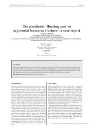
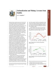
east <strong>coast</strong> <strong>of</strong> <strong>South</strong> <strong>Africa</strong> (Figure 1) experienced<br />
its largest recorded <str<strong>on</strong>g>wave</str<strong>on</strong>g> event in<br />
March 2007. <str<strong>on</strong>g>The</str<strong>on</strong>g> storm coincided with <strong>the</strong><br />
March equinox (highest astr<strong>on</strong>omical tide<br />
<strong>of</strong> <strong>the</strong> year) and had devastating effects <strong>on</strong><br />
<strong>the</strong> shoreline. C<strong>on</strong>sidering coincidence <strong>of</strong><br />
tide and significant <str<strong>on</strong>g>wave</str<strong>on</strong>g> height, <str<strong>on</strong>g>The</str<strong>on</strong>g>r<strong>on</strong> &<br />
Rossouw (2008) (cited by Wright (2009) and<br />
Smith et al (2010)) referred to <strong>the</strong> event as<br />
having a 500 year recurrence interval. Phelps<br />
et al (2009) found <strong>the</strong> recurrence interval <strong>of</strong><br />
<strong>the</strong> significant <str<strong>on</strong>g>wave</str<strong>on</strong>g> height to be between 34<br />
and 85 years, but noting that a 35 year occurrence<br />
was more likely. CSIR (2008) estimated<br />
<strong>the</strong> significant <str<strong>on</strong>g>wave</str<strong>on</strong>g> height return period<br />
<strong>of</strong> <strong>the</strong> storm to be 10 to 35 years, but noted<br />
that it was probably closer to a 10 year return<br />
period. Apart from <strong>the</strong> 500 year recurrence<br />
interval that c<strong>on</strong>siders <strong>the</strong> coincidence <strong>of</strong> <strong>the</strong><br />
tide and storm, <strong>the</strong> analysis <strong>of</strong> <strong>the</strong> significant<br />
<str<strong>on</strong>g>wave</str<strong>on</strong>g> height return period <strong>the</strong>refore ranges<br />
from 10 to 85 years. This wide range fur<strong>the</strong>r<br />
highlights <strong>the</strong> need for additi<strong>on</strong>al research<br />
<strong>on</strong> <strong>the</strong> characteristics <strong>of</strong> design <str<strong>on</strong>g>wave</str<strong>on</strong>g>s for <strong>the</strong><br />
east <strong>coast</strong> <strong>of</strong> <strong>South</strong> <strong>Africa</strong>.<br />
Once a <strong>coast</strong>al project has been designed<br />
in c<strong>on</strong>siderati<strong>on</strong> <strong>of</strong> a specific return period,<br />
<strong>the</strong> c<strong>on</strong>structi<strong>on</strong> or operati<strong>on</strong> <strong>of</strong> <strong>the</strong> project<br />
becomes <strong>the</strong> point <strong>of</strong> focus. C<strong>on</strong>structi<strong>on</strong><br />
and operati<strong>on</strong> <strong>of</strong> a development <strong>of</strong>ten<br />
depends <strong>on</strong> <strong>the</strong> exceedance statistics <strong>of</strong> a<br />
given <str<strong>on</strong>g>wave</str<strong>on</strong>g> parameter (see METHODS).<br />
Exceedance graphs are a tool used to identify<br />
<strong>the</strong> percentage <strong>of</strong> time a parameter will<br />
be exceeded. Exceedance statistics are not<br />
very useful to <strong>the</strong> design engineer, as <strong>the</strong><br />
probability <strong>of</strong> exceedance does not preclude<br />
dependent or related recordings <strong>of</strong> <strong>the</strong> same<br />
event. <str<strong>on</strong>g>The</str<strong>on</strong>g>refore this does not yield a recurrence<br />
interval estimate <strong>of</strong> independent storm<br />
events. Exceedance graphs are, however, <strong>of</strong><br />
value during <strong>coast</strong>al c<strong>on</strong>structi<strong>on</strong> work as a<br />
management tool. It allows <strong>the</strong> c<strong>on</strong>tractor,<br />
resident engineer or project manager to estimate<br />
how <strong>of</strong>ten work will be disrupted. For<br />
example, if a specific height <strong>of</strong> a c<strong>of</strong>ferdam is<br />
installed, exceedance statistics may be used<br />
to determine <strong>the</strong> probable number <strong>of</strong> days<br />
that <strong>the</strong> temporary works will be overtopped.<br />
TECHNICAL PAPER<br />
JOURNAL OF THE SOUTH AFRICAN<br />
INSTITUTION OF CIVIL ENGINEERING<br />
Vol 54 No 2, October 2012, Pages 45–54, Paper 809<br />
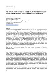
STEFANO CORBELLA (Member SAICE) received<br />
his BSc degree in civil engineering cum laude<br />
from <strong>the</strong> University <strong>of</strong> <strong>KwaZulu</strong>-<strong>Natal</strong>, <strong>South</strong><br />
<strong>Africa</strong>. He completed <strong>the</strong> requirements for an<br />
MSc in <strong>coast</strong>al engineering summa cum laude<br />
and is currently upgrading <strong>the</strong> MSc to a PhD. He<br />
is a practicing <strong>coast</strong>al engineer at <strong>the</strong> e<str<strong>on</strong>g>The</str<strong>on</strong>g>kwini<br />
Municipality’s Coastal Stormwater and<br />
Catchment Management Department.<br />
C<strong>on</strong>tact details:<br />
166 KE Masinga Road<br />
Durban<br />
4001<br />
<strong>South</strong> <strong>Africa</strong><br />
T: +27 31 311 7312<br />
E: corbellas@durban.gov.za<br />
PROF DEREK STRETCH is Pr<strong>of</strong>essor <strong>of</strong> Hydraulics<br />
and Envir<strong>on</strong>mental Fluid Mechanics at <strong>the</strong><br />
University <strong>of</strong> <strong>KwaZulu</strong>-<strong>Natal</strong>. He currently<br />
occupies <strong>the</strong> e<str<strong>on</strong>g>The</str<strong>on</strong>g>kwini-sp<strong>on</strong>sored Chair in Civil<br />
Engineering and is Director <strong>of</strong> <strong>the</strong> Centre for<br />
Research in Envir<strong>on</strong>mental, Coastal & Hydrological<br />
Engineering. His research group focuses <strong>on</strong> <strong>the</strong><br />
bio-hydrodynamics <strong>of</strong> estuarine systems, <strong>coast</strong>al<br />
and shoreline processes, and understanding turbulence and mixing in<br />
envir<strong>on</strong>mental flows.<br />
C<strong>on</strong>tact details:<br />
School <strong>of</strong> Engineering<br />
University <strong>of</strong> <strong>KwaZulu</strong>-<strong>Natal</strong><br />
Durban<br />
<strong>South</strong> <strong>Africa</strong><br />
4041<br />
T: +27 31 260 1064<br />
E: stretchd@ukzn.ac.za<br />
Key words: <str<strong>on</strong>g>wave</str<strong>on</strong>g> <str<strong>on</strong>g>climate</str<strong>on</strong>g>, <str<strong>on</strong>g>wave</str<strong>on</strong>g> data, <str<strong>on</strong>g>wave</str<strong>on</strong>g> parameter, <str<strong>on</strong>g>wave</str<strong>on</strong>g> roses,<br />
<strong>KwaZulu</strong>-<strong>Natal</strong> <strong>coast</strong>, <strong>coast</strong>al developments, seas<strong>on</strong>al trends<br />
Journal <strong>of</strong> <strong>the</strong> <strong>South</strong> <strong>Africa</strong>n Instituti<strong>on</strong> <strong>of</strong> Civil Engineering • Volume 54 Number 2 October 2012 45
<str<strong>on</strong>g>The</str<strong>on</strong>g> <str<strong>on</strong>g>wave</str<strong>on</strong>g> <str<strong>on</strong>g>climate</str<strong>on</strong>g> <strong>on</strong> <strong>the</strong> east <strong>coast</strong> <strong>of</strong><br />
<strong>South</strong> <strong>Africa</strong> has not been formally reviewed<br />
since Rossouw (1984) analysed existing <str<strong>on</strong>g>wave</str<strong>on</strong>g><br />
data for <strong>South</strong> <strong>Africa</strong>n and Namibian <strong>coast</strong>al<br />
waters. Rossouw c<strong>on</strong>cluded that <strong>on</strong>ly <strong>the</strong><br />
Waverider data (refer METHODS) is reliable<br />
enough to c<strong>on</strong>sider for design purposes. <str<strong>on</strong>g>The</str<strong>on</strong>g><br />
relatively l<strong>on</strong>g records <strong>of</strong> data (18 years) making<br />
up <strong>the</strong> current east <strong>coast</strong> record are from<br />
Durban and Richards Bay. Rossouw’s analysis<br />
was <strong>of</strong> a time when no <str<strong>on</strong>g>wave</str<strong>on</strong>g> recording buoys<br />
were operati<strong>on</strong>al in Durban. Durban’s reliable<br />
data has been analysed by various <strong>South</strong><br />
<strong>Africa</strong>n c<strong>on</strong>sultants and n<strong>on</strong>-commercial<br />
authors (examples include Van der Borch van<br />
Verwolde (2004) and Rossouw (2001)). This<br />
paper provides a re-analysis and update <strong>of</strong><br />
<strong>the</strong> <strong>KwaZulu</strong>-<strong>Natal</strong> <str<strong>on</strong>g>wave</str<strong>on</strong>g> recording data. It<br />
also places <strong>the</strong> analysed data into a formal<br />
design reference that is readily accessible.<br />
From a <strong>coast</strong>al design point <strong>of</strong> view<br />
<strong>the</strong>re was a need to identify what data was<br />
available for design applicati<strong>on</strong>s and how<br />
representative it was, since Durban’s record<br />
was made up <strong>of</strong> three different instruments<br />
at three different locati<strong>on</strong>s. Fortunately<br />
Richards Bay has a c<strong>on</strong>tinuous <str<strong>on</strong>g>wave</str<strong>on</strong>g> data set<br />
from its Waverider buoy that could be used<br />
to verify <strong>the</strong> results.<br />
Storm <str<strong>on</strong>g>wave</str<strong>on</strong>g>s are generated <strong>of</strong>f <strong>the</strong><br />
<strong>KwaZulu</strong>-<strong>Natal</strong> <strong>coast</strong> by tropical cycl<strong>on</strong>es,<br />
cold fr<strong>on</strong>ts or cut-<strong>of</strong>f lows. Cold fr<strong>on</strong>ts move<br />
from west to east and generally exist closer<br />
to <strong>the</strong> <strong>coast</strong> than cut-<strong>of</strong>f lows and cycl<strong>on</strong>es.<br />
Cold fr<strong>on</strong>ts occur more regularly than<br />
<strong>the</strong> o<strong>the</strong>r forcings and produce relatively<br />
smaller <str<strong>on</strong>g>wave</str<strong>on</strong>g> heights and <str<strong>on</strong>g>wave</str<strong>on</strong>g> periods<br />
with sou<strong>the</strong>rly directi<strong>on</strong>. Tropical cycl<strong>on</strong>es<br />
are rarely resp<strong>on</strong>sible for extreme <str<strong>on</strong>g>wave</str<strong>on</strong>g>s in<br />
Durban – between 1962 and 2005 <strong>on</strong>ly seven<br />
cycl<strong>on</strong>es affected <strong>the</strong> eastern parts <strong>of</strong> <strong>South</strong><br />
<strong>Africa</strong> (Kruger et al 2010). Generally tropical<br />
cycl<strong>on</strong>es produce north-easterly swells. Cut<strong>of</strong>f<br />
lows have been associated with <strong>the</strong> largest<br />
<str<strong>on</strong>g>wave</str<strong>on</strong>g> events <strong>on</strong> <strong>the</strong> <strong>KwaZulu</strong>-<strong>Natal</strong> <strong>coast</strong><br />
(March 2007). <str<strong>on</strong>g>The</str<strong>on</strong>g>y form fur<strong>the</strong>r <strong>of</strong>fshore<br />
than cold fr<strong>on</strong>ts and are generally associated<br />
with large south-easterly <str<strong>on</strong>g>wave</str<strong>on</strong>g>s with l<strong>on</strong>g<br />
<str<strong>on</strong>g>wave</str<strong>on</strong>g> periods. For a detailed descripti<strong>on</strong> <strong>of</strong><br />
<strong>South</strong> <strong>Africa</strong>n wea<strong>the</strong>r c<strong>on</strong>diti<strong>on</strong>s <strong>the</strong> reader<br />
is referred to Hunter (1987), Prest<strong>on</strong>-Whyte<br />
& Tys<strong>on</strong> (1993), and Taljaard (1995).<br />
This paper aims (1) to determine <strong>the</strong><br />
reliability <strong>of</strong> <strong>the</strong> Durban and Richards Bay<br />
Waverider data, and to use it to establish<br />
return periods <strong>of</strong> <str<strong>on</strong>g>wave</str<strong>on</strong>g> heights for <strong>the</strong> east<br />
<strong>coast</strong> <strong>of</strong> <strong>South</strong> <strong>Africa</strong>; (2) to present exceedance<br />
statistics <strong>of</strong> <str<strong>on</strong>g>wave</str<strong>on</strong>g> heights and peak<br />
period and to provide o<strong>the</strong>r typical <str<strong>on</strong>g>wave</str<strong>on</strong>g> statistics;<br />
and (3) to analyse <str<strong>on</strong>g>wave</str<strong>on</strong>g> height return<br />
periods by different methods to illustrate <strong>the</strong><br />
uncertainties and risks <strong>of</strong> basing designs <strong>on</strong> a<br />
short <str<strong>on</strong>g>wave</str<strong>on</strong>g> record.<br />
Namibia<br />
<strong>South</strong> <strong>Africa</strong><br />
<str<strong>on</strong>g>The</str<strong>on</strong>g> methods <strong>of</strong> analysis, as well as definiti<strong>on</strong>s<br />
<strong>of</strong> <strong>the</strong> <str<strong>on</strong>g>wave</str<strong>on</strong>g> parameters c<strong>on</strong>sidered,<br />
are described under METHODS. We <strong>the</strong>n<br />
present <strong>the</strong> exceedance statistics and o<strong>the</strong>r<br />
typical <str<strong>on</strong>g>wave</str<strong>on</strong>g> parameter statistics with seas<strong>on</strong>al<br />
variati<strong>on</strong>s. A discussi<strong>on</strong> <strong>of</strong> multivariate<br />
return periods is given prior to summarising<br />
<strong>the</strong> c<strong>on</strong>clusi<strong>on</strong>s.<br />
METHODS<br />
<str<strong>on</strong>g>The</str<strong>on</strong>g> first phase <strong>of</strong> <strong>the</strong> analysis was verifying<br />
<strong>the</strong> validity <strong>of</strong> <strong>the</strong> available data. Analysis <strong>of</strong><br />
<strong>the</strong> <str<strong>on</strong>g>wave</str<strong>on</strong>g> <str<strong>on</strong>g>climate</str<strong>on</strong>g> could <strong>the</strong>n be performed<br />
with respect to seas<strong>on</strong>al distributi<strong>on</strong>s, exceedance<br />
graphs, typical statistics, and a univariate<br />
statistical analysis <strong>of</strong> extreme <str<strong>on</strong>g>wave</str<strong>on</strong>g> heights.<br />
<str<strong>on</strong>g>The</str<strong>on</strong>g> <str<strong>on</strong>g>wave</str<strong>on</strong>g> parameters analysed included<br />
<strong>the</strong> significant <str<strong>on</strong>g>wave</str<strong>on</strong>g> height, Hs, which, in<br />
deep water, is equal to 4√m 0 where m o is <strong>the</strong><br />
area under <strong>the</strong> <str<strong>on</strong>g>wave</str<strong>on</strong>g> spectrum; <strong>the</strong> maximum<br />
<str<strong>on</strong>g>wave</str<strong>on</strong>g> height, H max , is <strong>the</strong> largest <str<strong>on</strong>g>wave</str<strong>on</strong>g><br />
recorded in a recording period; <strong>the</strong> peak<br />
period, T p , is <strong>the</strong> period at which <strong>the</strong><br />
maximum energy density occurs and is<br />
<strong>the</strong> inverse <strong>of</strong> <strong>the</strong> peak energy frequency f p ,<br />
T p = 1 ; and <strong>the</strong> <str<strong>on</strong>g>wave</str<strong>on</strong>g> directi<strong>on</strong> is <strong>the</strong> mean<br />
f p<br />
<str<strong>on</strong>g>wave</str<strong>on</strong>g> directi<strong>on</strong> measured from true north.<br />
Hs should be used to model <strong>coast</strong>al process<br />
and shoreline resp<strong>on</strong>se while H max is<br />
more appropriate to calculate <str<strong>on</strong>g>wave</str<strong>on</strong>g> loading<br />
<strong>on</strong> structures. T p is used to define <strong>the</strong> surf<br />
similarity parameter and is c<strong>on</strong>sequentially<br />
used to quantify <str<strong>on</strong>g>wave</str<strong>on</strong>g> run-up, scour and<br />
forces <strong>on</strong> structures (<strong>the</strong> larger <strong>the</strong> period,<br />
<strong>the</strong> larger <strong>the</strong> <str<strong>on</strong>g>wave</str<strong>on</strong>g> run-up and forces <strong>on</strong><br />
structures). An increase in period has also<br />
been shown to increase erosi<strong>on</strong> (Van Gent et<br />
al 2008; Van Thiel de Vries et al 2008).<br />
Validity <strong>of</strong> <strong>the</strong> <str<strong>on</strong>g>wave</str<strong>on</strong>g> data<br />
Durban’s 18 years <strong>of</strong> <str<strong>on</strong>g>wave</str<strong>on</strong>g> records are a combinati<strong>on</strong><br />
<strong>of</strong> three different <str<strong>on</strong>g>wave</str<strong>on</strong>g> recording<br />
<strong>KwaZulu</strong>-<br />
<strong>Natal</strong><br />
East Coast<br />
Waverider Richards Bay<br />
(1992–2010)<br />
ADCP (2002–2006)<br />
Waverider Durban<br />
(2007–2010)<br />
Figure 1 Map <strong>of</strong> <strong>South</strong> <strong>Africa</strong> showing <strong>KwaZulu</strong>-<strong>Natal</strong> with locati<strong>on</strong>s <strong>of</strong> Waverider buoys and ADCP<br />
W<br />
Waverider Durban (1992–2001)<br />
instruments at three different locati<strong>on</strong>s<br />
(Table 1), two Waverider buoys and an<br />
acoustic doppler current pr<strong>of</strong>iler (ADCP).<br />
Waverider, which is <strong>the</strong> trade name <strong>of</strong><br />
Datawell’s <str<strong>on</strong>g>wave</str<strong>on</strong>g> recording buoy, is a spherical<br />
accelerometer buoy that calculates <str<strong>on</strong>g>wave</str<strong>on</strong>g><br />
heights from accelerati<strong>on</strong>s. <str<strong>on</strong>g>The</str<strong>on</strong>g> ADCP is<br />
located <strong>on</strong> <strong>the</strong> ocean floor and uses s<strong>on</strong>ar to<br />
measure <str<strong>on</strong>g>wave</str<strong>on</strong>g> heights.<br />
<str<strong>on</strong>g>The</str<strong>on</strong>g> different locati<strong>on</strong>s were a c<strong>on</strong>cern<br />
because <strong>of</strong> <strong>the</strong> shoaling and refracti<strong>on</strong> effects<br />
<strong>of</strong> <strong>the</strong> different water depths. Diedericks<br />
(2009) found that <strong>the</strong> Richards Bay data<br />
has a good correlati<strong>on</strong> with Durban’s data.<br />
Diedericks’ findings were verified by finding<br />
a Pears<strong>on</strong> correlati<strong>on</strong> coefficient and a ratio<br />
between <strong>the</strong> Durban Waverider buoy and <strong>the</strong><br />
Richards Bay Waverider buoy, and between<br />
<strong>the</strong> Durban ADCP and <strong>the</strong> Richards Bay<br />
Waverider buoy (Table 5).<br />
<str<strong>on</strong>g>The</str<strong>on</strong>g>re was still a c<strong>on</strong>cern that <strong>the</strong> ADCP<br />
data was not representative enough <strong>of</strong> deepwater<br />
<str<strong>on</strong>g>wave</str<strong>on</strong>g> c<strong>on</strong>diti<strong>on</strong>s and so <strong>the</strong> recorded<br />
<str<strong>on</strong>g>wave</str<strong>on</strong>g>s were classified as ei<strong>the</strong>r deep water,<br />
transiti<strong>on</strong>al or shallow water by c<strong>on</strong>sidering<br />
<strong>the</strong> range <strong>of</strong> <strong>the</strong>ir depth over <str<strong>on</strong>g>wave</str<strong>on</strong>g> length<br />
ratio (Table 2). Newt<strong>on</strong>’s method was used to<br />
iteratively solve <strong>the</strong> <str<strong>on</strong>g>wave</str<strong>on</strong>g> length L using <strong>the</strong><br />
peak <str<strong>on</strong>g>wave</str<strong>on</strong>g> period T p , depth h and gravitati<strong>on</strong>al<br />
accelerati<strong>on</strong> g (Equati<strong>on</strong> 1).<br />
x 2 = x 1 – y(x 1 )<br />
y’(x 1 ) = x 1 – x 1 – Dcoth(x 1 )<br />
1 + D(coth 2 x 1 –1)<br />
where<br />
(1)<br />
D = 4π2 h 2πh<br />
and x = , is <strong>the</strong> <str<strong>on</strong>g>wave</str<strong>on</strong>g> number<br />
gTp2 L<br />
It was decided that since <strong>the</strong> ADCP did not<br />
record <strong>the</strong> 2007 event, in additi<strong>on</strong> to being<br />
in much shallower water than <strong>the</strong> o<strong>the</strong>r<br />
instruments, this entire data set would be<br />
replaced by <strong>the</strong> Richards Bay data which had<br />
a str<strong>on</strong>g correlati<strong>on</strong> to <strong>the</strong> Durban Waverider<br />
buoys. <str<strong>on</strong>g>The</str<strong>on</strong>g> Richards Bay data is a c<strong>on</strong>tinuous<br />
N<br />
S<br />
E<br />
46<br />
Journal <strong>of</strong> <strong>the</strong> <strong>South</strong> <strong>Africa</strong>n Instituti<strong>on</strong> <strong>of</strong> Civil Engineering • Volume 54 Number 2 October 2012
Table 1 Historical <str<strong>on</strong>g>wave</str<strong>on</strong>g> recording instruments,<br />
<strong>the</strong>ir operating periods and water depth<br />
Instrument<br />
Date<br />
Depth<br />
(m)<br />
Durban Waverider 1992–2001 42<br />
Durban ADCP 2002–2006 15<br />
Durban Waverider 2007–2009 30<br />
Richards Bay Waverider 1992–2009 22<br />
Table 2 Classificati<strong>on</strong> <strong>of</strong> water <str<strong>on</strong>g>wave</str<strong>on</strong>g>s by <strong>the</strong><br />
ratio <strong>of</strong> water depth d to <strong>the</strong> <str<strong>on</strong>g>wave</str<strong>on</strong>g><br />
length L (Adapted from U.S. Army<br />
Corps <strong>of</strong> Engineers, 2006).<br />
Deep water<br />
Classificati<strong>on</strong><br />
d/L (m/m)<br />
1/2 to ∞<br />
Transiti<strong>on</strong>al 1/20 to 1/2<br />
Shallow water 0 to 1/20<br />
Table 3 Seas<strong>on</strong>al definiti<strong>on</strong> <strong>of</strong> m<strong>on</strong>ths<br />
Seas<strong>on</strong><br />
M<strong>on</strong>ths<br />
Summer 12 to 2<br />
Autumn 3 to 5<br />
Winter 6 to 8<br />
Spring 9 to 11<br />
set from a c<strong>on</strong>stant locati<strong>on</strong>, and so it was<br />
also analysed to c<strong>on</strong>firm and compare <strong>the</strong><br />
Durban results. Unfortunately Richards Bay<br />
was not without its limitati<strong>on</strong>s and, although<br />
it recorded <strong>the</strong> 2007 event, it did not record<br />
<strong>the</strong> sec<strong>on</strong>d and third largest events. <str<strong>on</strong>g>The</str<strong>on</strong>g>se<br />
events had to be incorporated into <strong>the</strong><br />
Richards Bay data from <strong>the</strong> Durban records.<br />
Seas<strong>on</strong>al distributi<strong>on</strong> <strong>of</strong><br />
<str<strong>on</strong>g>wave</str<strong>on</strong>g> parameters<br />
Each data set was analysed independently to<br />
establish if <strong>the</strong>re were any inc<strong>on</strong>sistencies or<br />
biases. <str<strong>on</strong>g>The</str<strong>on</strong>g> sets were analysed annually and<br />
seas<strong>on</strong>ally. <str<strong>on</strong>g>The</str<strong>on</strong>g> m<strong>on</strong>ths were divided into<br />
seas<strong>on</strong>s using <strong>the</strong> meteorological c<strong>on</strong>venti<strong>on</strong><br />
as defined in Table 3.<br />
All <strong>the</strong> recordings were counted and used<br />
to determine what percentage <strong>of</strong> a specific<br />
seas<strong>on</strong> and year made up a data set. <str<strong>on</strong>g>The</str<strong>on</strong>g> data<br />
sets were made up <strong>of</strong> measurements at threehour<br />
intervals, which means that a seas<strong>on</strong><br />
may c<strong>on</strong>tribute a larger percentage to <strong>the</strong> data<br />
set in terms <strong>of</strong> data points, but be missing a<br />
significant amount <strong>of</strong> days <strong>of</strong> data. This problem<br />
was resolved by calculating a percentage<br />
<strong>of</strong> days missing. <str<strong>on</strong>g>The</str<strong>on</strong>g> percentage <strong>of</strong> data and<br />
<strong>the</strong> percentage <strong>of</strong> days missing showed which<br />
seas<strong>on</strong>s or years had <strong>the</strong> potential to skew<br />
results or create bias, and identified which<br />
periods needed to be supplemented by <strong>the</strong><br />
o<strong>the</strong>r data set. A few days <strong>of</strong> missing data was<br />
deemed to be insignificant, if not during a<br />
storm event, but m<strong>on</strong>ths to years <strong>of</strong> missing<br />
data was supplemented.<br />
Average directi<strong>on</strong> was <strong>on</strong>ly available from<br />
<strong>the</strong> Durban ADCP (2002 – 2006) and <strong>the</strong><br />
Durban Waverider (2007 – 2009), making<br />
H max , Hs and T p <strong>the</strong> <strong>on</strong>ly parameters analysed<br />
for <strong>the</strong> full 18 years <strong>of</strong> data. <str<strong>on</strong>g>The</str<strong>on</strong>g> Richards Bay<br />
data had <str<strong>on</strong>g>wave</str<strong>on</strong>g> directi<strong>on</strong>s from 1997 to 2009,<br />
but differed from <strong>the</strong> Durban data as a result<br />
<strong>of</strong> different local wind c<strong>on</strong>diti<strong>on</strong>s.<br />
Exceedance graphs<br />
Supplementing Durban’s data with Richards<br />
Bay’s data created an 18 year data set for<br />
Durban. Exceedance graphs were created for<br />
Hs, H max and T p for each <strong>of</strong> <strong>the</strong> four seas<strong>on</strong>s.<br />
<str<strong>on</strong>g>The</str<strong>on</strong>g> exceedance graphs provided an initial<br />
idea <strong>of</strong> event occurrences and allowed an<br />
Hs value to be selected for <strong>the</strong> peak-overthreshold<br />
method.<br />
<str<strong>on</strong>g>The</str<strong>on</strong>g> exceedance graphs were created by<br />
binning <strong>the</strong> parameter in questi<strong>on</strong> and <strong>the</strong>n<br />
calculating <strong>the</strong> frequency <strong>of</strong> occurrence per<br />
bin. <str<strong>on</strong>g>The</str<strong>on</strong>g> frequencies were <strong>the</strong>n used to find<br />
<strong>the</strong> frequency <strong>of</strong> events that exceeded each<br />
bin. <str<strong>on</strong>g>The</str<strong>on</strong>g> exceedance frequencies were <strong>the</strong>n<br />
divided by <strong>the</strong> total number <strong>of</strong> data points<br />
and expressed as a percentage exceedance.<br />
<str<strong>on</strong>g>The</str<strong>on</strong>g> parameters were plotted against <strong>the</strong> percentage<br />
<strong>on</strong> a log scale to produce <strong>the</strong> exceedance<br />
graphs. A best fit line was <strong>the</strong>n used to<br />
interpret <strong>the</strong> percentage <strong>of</strong> time a given <str<strong>on</strong>g>wave</str<strong>on</strong>g><br />
height is equalled or exceeded.<br />
Wave <str<strong>on</strong>g>climate</str<strong>on</strong>g> variati<strong>on</strong><br />
and typical statistics<br />
<str<strong>on</strong>g>The</str<strong>on</strong>g> following parameters were extracted<br />
from <strong>the</strong> data set annually and seas<strong>on</strong>ally:<br />
<strong>the</strong> maximum H max , Hs, T p , and <strong>the</strong> average<br />
T p , Hs and <str<strong>on</strong>g>wave</str<strong>on</strong>g> directi<strong>on</strong>. Comparing <strong>the</strong><br />
parameters seas<strong>on</strong>ally illustrated <strong>the</strong> degree<br />
<strong>of</strong> seas<strong>on</strong>al variati<strong>on</strong>.<br />
<str<strong>on</strong>g>The</str<strong>on</strong>g> average <str<strong>on</strong>g>wave</str<strong>on</strong>g> directi<strong>on</strong> was calculated,<br />
as well as <strong>the</strong> significant <str<strong>on</strong>g>wave</str<strong>on</strong>g> height<br />
weighted average directi<strong>on</strong>. <str<strong>on</strong>g>The</str<strong>on</strong>g> results differed<br />
negligibly, so <strong>on</strong>ly <strong>the</strong> weighted average<br />
directi<strong>on</strong>s are presented.<br />
Since minor events had <strong>the</strong> potential <strong>of</strong><br />
dampening major events in specific seas<strong>on</strong>s,<br />
<strong>the</strong> analysis <strong>of</strong> <strong>the</strong> Hs data was also d<strong>on</strong>e<br />
<strong>on</strong>ly c<strong>on</strong>sidering events exceeding 3.5 m<br />
<str<strong>on</strong>g>wave</str<strong>on</strong>g> heights.<br />
Univariate statistical analysis<br />
<strong>of</strong> extreme <str<strong>on</strong>g>wave</str<strong>on</strong>g>s<br />
<str<strong>on</strong>g>The</str<strong>on</strong>g> average recurrence interval or return<br />
period <strong>of</strong> independent <str<strong>on</strong>g>wave</str<strong>on</strong>g> events can be<br />
estimated by fitting a <strong>the</strong>oretical probability<br />
distributi<strong>on</strong> to <strong>the</strong> data and using it to<br />
extrapolate to <strong>the</strong> event <strong>of</strong> interest. <str<strong>on</strong>g>The</str<strong>on</strong>g>re are<br />
many available probability distributi<strong>on</strong>s, and<br />
<strong>the</strong> use <strong>of</strong> an appropriate <strong>on</strong>e is important to<br />
accurately model <strong>the</strong> data and to realistically<br />
estimate <strong>the</strong> probability <strong>of</strong> rare events by<br />
extrapolati<strong>on</strong>.<br />
<str<strong>on</strong>g>The</str<strong>on</strong>g> literature identifies comm<strong>on</strong>ly used<br />
distributi<strong>on</strong>s, but does not state which is<br />
preferred or superior. <str<strong>on</strong>g>The</str<strong>on</strong>g> U.S. Army Corps<br />
<strong>of</strong> Engineers (1985, 2006) recommends <strong>the</strong><br />
guidelines <strong>of</strong> Isaacs<strong>on</strong> & Mckensie (1981) while<br />
providing guidelines for <strong>the</strong> Extremal Type I<br />
(Fisher Tippett I) distributi<strong>on</strong> and also recommends<br />
Fisher Tippett II. Isaacs<strong>on</strong> & Mckensie<br />
(1981) provide guidelines for <strong>the</strong> Lognormal,<br />
Extremal Type I and II, and <strong>the</strong> Weibull distributi<strong>on</strong>.<br />
Chadwick et al (2004) noted that <strong>the</strong><br />
Department <strong>of</strong> Energy recommends using <strong>the</strong><br />
Gumbel, Fisher Tippett I or <strong>the</strong> Extremal Value<br />
Type I distributi<strong>on</strong>. Goda (2008) provides<br />
guidelines for <strong>the</strong> use <strong>of</strong> <strong>the</strong> Fisher-Tippett<br />
I, Fisher-Tippett II, Weibull and Lognormal<br />
distributi<strong>on</strong>s. <str<strong>on</strong>g>The</str<strong>on</strong>g> Generalised Extreme<br />
Value distributi<strong>on</strong> (GEV) encompasses <strong>the</strong><br />
Fisher-Tippet distributi<strong>on</strong>s, and <strong>the</strong> Extreme<br />
Value distributi<strong>on</strong> is equivalent to <strong>the</strong> Gumbel<br />
distributi<strong>on</strong>. <str<strong>on</strong>g>The</str<strong>on</strong>g> GEV distributi<strong>on</strong> has been<br />
used extensively for extreme value analysis <strong>of</strong><br />
hydrological events and specifically for <str<strong>on</strong>g>wave</str<strong>on</strong>g><br />
heights by Guedes Soares & Scotto (2004) and<br />
Chini et al (2010), while <strong>the</strong> Generalised Pareto<br />
(GP) distributi<strong>on</strong> has been used by Callaghan<br />
et al (2008) and Hawkes (2002). Ruggiero et<br />
al (2010) c<strong>on</strong>sidered both <strong>the</strong> GP and GEV<br />
distributi<strong>on</strong>s. C<strong>on</strong>sidering <strong>the</strong> above sources,<br />
<strong>the</strong> Weibull, Lognormal, Generalised Pareto,<br />
Extreme Value and <strong>the</strong> Generalised Extreme<br />
Value distributi<strong>on</strong>s were used in <strong>the</strong> analysis.<br />
Probability density functi<strong>on</strong>s:<br />
Weibull<br />
y = kσ –k x k–1 e – <br />
x<br />
σ<br />
: 0 ≤ x < ∞<br />
k<br />
<br />
Extreme value (GEV1 or Gumbel)<br />
y = σ –1 e – x–μ<br />
σ<br />
: –∞ < x < ∞<br />
Lognormal<br />
y =<br />
ke –e x–μ<br />
σ<br />
–(lnx–μ)<br />
1<br />
2<br />
xσ√2π e 2σ 2<br />
: 0 < x < ∞<br />
<br />
Generalised extreme value<br />
y = <br />
1<br />
σ<br />
: 1 + k<br />
e – 1+k (x–μ) –1 k<br />
σ<br />
1+k(x–μ) –1– 1 k<br />
σ<br />
<br />
<br />
<br />
(x – μ)<br />
σ<br />
> 0<br />
<br />
<br />
<br />
Journal <strong>of</strong> <strong>the</strong> <strong>South</strong> <strong>Africa</strong>n Instituti<strong>on</strong> <strong>of</strong> Civil Engineering • Volume 54 Number 2 October 2012 47
Generalised Pareto<br />
Table 4 <str<strong>on</strong>g>The</str<strong>on</strong>g> percentage <strong>of</strong> different water <str<strong>on</strong>g>wave</str<strong>on</strong>g>s recorded by <strong>the</strong> various recording instruments<br />
y = <br />
1<br />
σ<br />
– θ) –1–<br />
1 + k(x<br />
1 k<br />
σ<br />
<br />
: θ < x, for k > 0<br />
σ<br />
: θ < x < –<br />
k , for k < 0<br />
<br />
where μ is <strong>the</strong> locati<strong>on</strong> parameter, σ is <strong>the</strong><br />
scale parameter, k is <strong>the</strong> shape parameter.<br />
Data Set<br />
Durban Waverider<br />
(1992–2001)<br />
Durban ADCP<br />
(2002–2006)<br />
Durban Waverider<br />
(2007–2009)<br />
Richards Bay Waverider<br />
(1992–2009)<br />
Water Depth<br />
(m)<br />
Deep Water<br />
Waves (%)<br />
Transiti<strong>on</strong> Water<br />
Waves (%)<br />
Shallow Water<br />
Waves (%)<br />
42 22.7 77.3 0.0<br />
15 0.2 99.7 0.1<br />
30 10.1 89.9 0.0<br />
22 2.2 97.8 0.0<br />
<str<strong>on</strong>g>The</str<strong>on</strong>g>re are numerous fitting methods available,<br />
but probably <strong>the</strong> most popular is <strong>the</strong> maximum<br />
likelihood. <str<strong>on</strong>g>The</str<strong>on</strong>g> method maximises <strong>the</strong><br />
probability <strong>of</strong> observing <strong>the</strong> data set that has<br />
been observed in <strong>the</strong> sample. This intuitive<br />
approach has led to <strong>the</strong> method being referred<br />
to as <strong>the</strong> most popular and best technique for<br />
deriving estimators (Casella & Berger 1990;<br />
M<strong>on</strong>tgomery & Runger 2003). <str<strong>on</strong>g>The</str<strong>on</strong>g> maximum<br />
likelihood method is popular with statisticians<br />
as its characteristics can be examined<br />
ma<strong>the</strong>matically (Goda 2008). It shows a small<br />
amount <strong>of</strong> negative bias, but seems to have <strong>the</strong><br />
smallest degree <strong>of</strong> deviati<strong>on</strong> (Goda 2008). <str<strong>on</strong>g>The</str<strong>on</strong>g><br />
method requires lengthy iterative manipulati<strong>on</strong><br />
(Isaacs<strong>on</strong> & MacKensie 1981), an issue<br />
that has largely been removed with modern<br />
computing capabilities. <str<strong>on</strong>g>The</str<strong>on</strong>g> maximum likelihood<br />
method is <strong>the</strong>refore used in this study.<br />
<str<strong>on</strong>g>The</str<strong>on</strong>g> Akaike informati<strong>on</strong> criteri<strong>on</strong> (Equati<strong>on</strong> 2)<br />
was used to determine <strong>the</strong> best fitting probability<br />
distributi<strong>on</strong>.<br />
AIC = 2k – 2ln (L) (2)<br />
where k is <strong>the</strong> number <strong>of</strong> parameters in <strong>the</strong><br />
probability distributi<strong>on</strong> and L is <strong>the</strong> maximised<br />
value <strong>of</strong> <strong>the</strong> likelihood functi<strong>on</strong> for <strong>the</strong><br />
estimated parameters.<br />
<str<strong>on</strong>g>The</str<strong>on</strong>g> length <strong>of</strong> <strong>the</strong> <str<strong>on</strong>g>wave</str<strong>on</strong>g> data record<br />
was <strong>on</strong>ly 18 years and so it was decided<br />
to statistically analyse <strong>the</strong> H max and Hs<br />
<str<strong>on</strong>g>wave</str<strong>on</strong>g> heights with both <strong>the</strong> annual maxima<br />
method and peak-over-threshold method<br />
(POT). <str<strong>on</strong>g>The</str<strong>on</strong>g> peak-over-threshold method was<br />
<strong>on</strong>ly applied to <strong>the</strong> Hs data for a threshold <strong>of</strong><br />
3.5 m. When performing <strong>the</strong> POT method<br />
it is imperative that <strong>on</strong>ly independent events<br />
are c<strong>on</strong>sidered. To ensure this, data was<br />
divided into events using <strong>the</strong> following definiti<strong>on</strong>:<br />
a storm event commences when Hs<br />
exceeds 3.5 m and ends when Hs falls below<br />
3.5 m, and remains below for approximately<br />
<strong>on</strong>e m<strong>on</strong>th, based <strong>on</strong> <strong>the</strong> decay time <strong>of</strong> <strong>the</strong><br />
autocorrelati<strong>on</strong>. <str<strong>on</strong>g>The</str<strong>on</strong>g> Richards Bay data was<br />
similarly analysed.<br />
<str<strong>on</strong>g>The</str<strong>on</strong>g> 95% c<strong>on</strong>fidence intervals were found<br />
for <strong>the</strong> return periods using bootstrapping.<br />
Bootstrapping is a resampling technique with<br />
replacement. <str<strong>on</strong>g>The</str<strong>on</strong>g> bootstrapped samples were<br />
used to calculate <strong>the</strong> critical t statistic, which<br />
was in turn used to bound <strong>the</strong> estimated<br />
Table 5 Pears<strong>on</strong> correlati<strong>on</strong>, standard deviati<strong>on</strong> and ratio between different instrument-recorded Hs<br />
Data Sets<br />
Durban Waverider (1992–2001) vs<br />
Richards Bay Waverider (1992–2009)<br />
Durban ADCP (2002–2006) vs<br />
Richards Bay Waverider (1992–2009)<br />
Hs (m)<br />
6<br />
5<br />
4<br />
3<br />
2<br />
1<br />
0<br />
0<br />
return intervals. For a given value μ <strong>of</strong> a<br />
sample <strong>the</strong>re is a probability (1–α) <strong>of</strong> selecting<br />
a sample for which <strong>the</strong> c<strong>on</strong>fidence interval<br />
will c<strong>on</strong>tain <strong>the</strong> true value <strong>of</strong> μ. <str<strong>on</strong>g>The</str<strong>on</strong>g> 100(1–α)<br />
percent c<strong>on</strong>fidence interval for <strong>the</strong> t distributi<strong>on</strong><br />
is given by Equati<strong>on</strong> 3.<br />
x‒ – t α/2,n–1 s<br />
≤ μ ≤ x ‒ + t α/2,n–1 s<br />
(3)<br />
√n<br />
√n<br />
where x‒ is <strong>the</strong> mean <strong>of</strong> <strong>the</strong> bootstrapped<br />
sample, s is <strong>the</strong> standard deviati<strong>on</strong>, n is <strong>the</strong><br />
Correlati<strong>on</strong><br />
(Pears<strong>on</strong>)<br />
Average<br />
Ratio <strong>of</strong> Hs<br />
Standard<br />
Deviati<strong>on</strong><br />
0.84 1.08 0.25<br />
0.77 0.85 0.28<br />
400<br />
Hours<br />
Figure 2 Comparis<strong>on</strong> <strong>of</strong> Richards Bay’s Waverider (×) and Durban’s Waverider (●) during May 1998<br />
Hs (m)<br />
6<br />
5<br />
4<br />
3<br />
2<br />
1<br />
0<br />
0<br />
100<br />
100<br />
200<br />
200<br />
300<br />
300<br />
400<br />
Hours<br />
Figure 3 Comparis<strong>on</strong> <strong>of</strong> Richards Bay’s Waverider (×) and Durban’s ADCP (●) during July 2002<br />
500<br />
500<br />
600<br />
600<br />
700<br />
700<br />
800<br />
800<br />
number <strong>of</strong> samples and t α/2,n–1 is <strong>the</strong> upper<br />
100α/2 percentage point <strong>of</strong> <strong>the</strong> t distributi<strong>on</strong><br />
with n–1 degrees <strong>of</strong> freedom.<br />
RESULTS<br />
<str<strong>on</strong>g>The</str<strong>on</strong>g> Richards Bay data is shown to be a<br />
representative measure <strong>of</strong> <strong>the</strong> Durban <str<strong>on</strong>g>wave</str<strong>on</strong>g><br />
c<strong>on</strong>diti<strong>on</strong>s. <str<strong>on</strong>g>The</str<strong>on</strong>g> two data sets are used in<br />
c<strong>on</strong>juncti<strong>on</strong> to establish exceedance probabilities,<br />
typical <str<strong>on</strong>g>wave</str<strong>on</strong>g> parameter statistics,<br />
48<br />
Journal <strong>of</strong> <strong>the</strong> <strong>South</strong> <strong>Africa</strong>n Instituti<strong>on</strong> <strong>of</strong> Civil Engineering • Volume 54 Number 2 October 2012
North<br />
North<br />
North<br />
20%<br />
15%<br />
20%<br />
West<br />
15%<br />
10%<br />
5%<br />
East<br />
West<br />
5%<br />
10%<br />
East<br />
West<br />
15%<br />
10%<br />
5%<br />
East<br />
<strong>South</strong><br />
(a)<br />
<strong>South</strong><br />
(b)<br />
<strong>South</strong><br />
(c)<br />
4.5–9 3.5–4.5 2.5–3.5 2–2.5 1.75–2 1.5–1.75 1.25–1.5 1–1.25 0.75–1 < 0.75<br />
Figure 4 Comparis<strong>on</strong> <strong>of</strong> <strong>the</strong> entire data set <str<strong>on</strong>g>wave</str<strong>on</strong>g> roses for (a) Durban Waverider (2007–2009), (b) Durban ADCP (2002–2006) and (c) Richards Bay<br />
Waverider (1997–2009)<br />
seas<strong>on</strong>al trends and average recurrence<br />
intervals <strong>of</strong> <str<strong>on</strong>g>wave</str<strong>on</strong>g> heights al<strong>on</strong>g <strong>the</strong> east <strong>coast</strong><br />
<strong>of</strong> <strong>South</strong> <strong>Africa</strong>.<br />
Wave data validity<br />
<str<strong>on</strong>g>The</str<strong>on</strong>g> <str<strong>on</strong>g>wave</str<strong>on</strong>g> data showed that <strong>the</strong> Richards Bay<br />
data was an acceptable supplement to <strong>the</strong><br />
Durban <str<strong>on</strong>g>wave</str<strong>on</strong>g> data. <str<strong>on</strong>g>The</str<strong>on</strong>g> <str<strong>on</strong>g>wave</str<strong>on</strong>g>s recorded from<br />
all <strong>the</strong> recording instruments were largely<br />
transiti<strong>on</strong>al water <str<strong>on</strong>g>wave</str<strong>on</strong>g>s (Table 4). <str<strong>on</strong>g>The</str<strong>on</strong>g><br />
Durban Waveriders, being in deeper water,<br />
recorded <strong>the</strong> most deep water <str<strong>on</strong>g>wave</str<strong>on</strong>g>s and,<br />
although <strong>the</strong> Richards Bay Waverider data<br />
c<strong>on</strong>sisted <strong>of</strong> <strong>on</strong>ly 2% deep water <str<strong>on</strong>g>wave</str<strong>on</strong>g>s, it was<br />
still ten times larger than <strong>the</strong> ADCP, making<br />
Richards Bay’s recorded <str<strong>on</strong>g>wave</str<strong>on</strong>g>s more similar<br />
to that <strong>of</strong> <strong>the</strong> Durban Waveriders than <strong>the</strong><br />
ADCP.<br />
Richards Bay’s Waverider showed a<br />
str<strong>on</strong>ger correlati<strong>on</strong> between <strong>the</strong> Durban<br />
Waverider than <strong>the</strong> ADCP (Table 5). When<br />
comparing <strong>the</strong> average ratios <strong>of</strong> significant<br />
<str<strong>on</strong>g>wave</str<strong>on</strong>g> heights, <strong>the</strong> Richards Bay data showed<br />
a 1.08 ratio with Durban’s Waverider data,<br />
while <strong>on</strong>ly a 0.85 with <strong>the</strong> ADCP data.<br />
<str<strong>on</strong>g>The</str<strong>on</strong>g> final justificati<strong>on</strong> in replacing <strong>the</strong><br />
ADCP data is shown in Figures 2 and 3.<br />
<str<strong>on</strong>g>The</str<strong>on</strong>g>se time series plots <strong>of</strong> <strong>the</strong> largest <str<strong>on</strong>g>wave</str<strong>on</strong>g><br />
events (overlapping <strong>the</strong> data sets) illustrate<br />
that <strong>the</strong> Richards Bay data is more representative<br />
<strong>of</strong> <strong>the</strong> Durban Waverider than <strong>the</strong><br />
Durban ADCP.<br />
Figure 4 shows a comparis<strong>on</strong> <strong>of</strong> <strong>the</strong><br />
<str<strong>on</strong>g>wave</str<strong>on</strong>g> roses for <strong>the</strong> entire data sets <strong>of</strong> <strong>the</strong><br />
Durban Waverider (2007–2009), <strong>the</strong> Durban<br />
ADCP (2002–2006) and <strong>the</strong> Richards Bay<br />
Waverider (1997–2009). <str<strong>on</strong>g>The</str<strong>on</strong>g> Durban and<br />
Richards Bay Waveriders show a similar<br />
sou<strong>the</strong>rly distributi<strong>on</strong> reaffirming <strong>the</strong><br />
str<strong>on</strong>g representati<strong>on</strong> <strong>of</strong> <strong>on</strong>e ano<strong>the</strong>r. <str<strong>on</strong>g>The</str<strong>on</strong>g><br />
Durban ADCP has a dominant easterly<br />
comp<strong>on</strong>ent and is essentially <strong>the</strong> result<br />
<strong>of</strong> refracti<strong>on</strong> occurring at <strong>the</strong> ADCP’s<br />
shallow depth.<br />
Table 6 Intercepts and slopes <strong>of</strong> significant <str<strong>on</strong>g>wave</str<strong>on</strong>g> height exceedance regressi<strong>on</strong> lines for summer,<br />
autumn, winter and spring, and <strong>the</strong>ir associated R 2 values. <str<strong>on</strong>g>The</str<strong>on</strong>g> bracketed values show <strong>the</strong><br />
95% c<strong>on</strong>fidence intervals<br />
Seas<strong>on</strong> Intercept Slope R 2<br />
Summer 1.21 (1.01; 1.42) –0.37 (–0.41; –0.33) 0.99<br />
Autumn 0.82 (0.54; 1.09) –0.68 (–0.73; –0.64) 0.99<br />
Winter 1.25 (1.04; 1.46) –0.45 (–0.49; –0.41) 0.99<br />
Spring 1.24 (1.01; 1.46) –0.45 (–0.50; –0.41) 0.99<br />
Hs (m)<br />
9<br />
8<br />
7<br />
6<br />
5<br />
4<br />
3<br />
2<br />
1<br />
0<br />
100<br />
Figure 5 Significant <str<strong>on</strong>g>wave</str<strong>on</strong>g> height (Hs) percentage exceedance for summer (■), autumn (▲), winter<br />
(×) and spring (+) (refer Table 6 for regressi<strong>on</strong> parameters)<br />
C<strong>on</strong>sequently <strong>the</strong> Richards Bay data was<br />
substituted for <strong>the</strong> ADCP data and used to<br />
supplement o<strong>the</strong>r missing data points, and a<br />
complete 18-year data set was attained.<br />
<str<strong>on</strong>g>The</str<strong>on</strong>g> Richards Bay data <strong>on</strong> <strong>the</strong> o<strong>the</strong>r hand<br />
was a c<strong>on</strong>tinuous set from <strong>the</strong> same locati<strong>on</strong>,<br />
having <str<strong>on</strong>g>wave</str<strong>on</strong>g> directi<strong>on</strong> recordings from 1997.<br />
<str<strong>on</strong>g>The</str<strong>on</strong>g> Richards Bay data did c<strong>on</strong>tain minor<br />
gaps and Durban’s data was used to supplement<br />
two missing <str<strong>on</strong>g>wave</str<strong>on</strong>g> events. <str<strong>on</strong>g>The</str<strong>on</strong>g> Richards<br />
Bay data was analysed to compare and verify<br />
<strong>the</strong> results <strong>of</strong> <strong>the</strong> Durban data.<br />
10 1 0.1 0.01<br />
Percentage Exceedance<br />
Exceedance probabilities<br />
and <str<strong>on</strong>g>wave</str<strong>on</strong>g> roses<br />
As previously menti<strong>on</strong>ed, exceedance graphs<br />
are not useful in a design applicati<strong>on</strong>, but are<br />
valuable in project planning.<br />
<str<strong>on</strong>g>The</str<strong>on</strong>g> exceedance graphs are shown seas<strong>on</strong>ally.<br />
Figure 5 shows an exceedance graph<br />
<strong>of</strong> significant <str<strong>on</strong>g>wave</str<strong>on</strong>g> height (Hs) and Figure 6<br />
shows an exceedance graph <strong>of</strong> maximum<br />
<str<strong>on</strong>g>wave</str<strong>on</strong>g> height (H max ). Wave directi<strong>on</strong> barely<br />
shows a seas<strong>on</strong>al variati<strong>on</strong> and it is presented<br />
as <str<strong>on</strong>g>wave</str<strong>on</strong>g> roses in Figure 8.<br />
Journal <strong>of</strong> <strong>the</strong> <strong>South</strong> <strong>Africa</strong>n Instituti<strong>on</strong> <strong>of</strong> Civil Engineering • Volume 54 Number 2 October 2012 49
Figures 5 and 6 show that autumn experiences<br />
<strong>the</strong> largest <str<strong>on</strong>g>wave</str<strong>on</strong>g>s followed by winter<br />
and spring and <strong>the</strong>n summer. Autumn,<br />
with regard to <str<strong>on</strong>g>wave</str<strong>on</strong>g> height exceedance (Hs<br />
and H max ), is <strong>the</strong> <strong>on</strong>ly seas<strong>on</strong> that shows a<br />
significant statistical difference from <strong>the</strong><br />
o<strong>the</strong>r seas<strong>on</strong>s at a 95% c<strong>on</strong>fidence limit.<br />
Based <strong>on</strong> <strong>the</strong> available data, <str<strong>on</strong>g>wave</str<strong>on</strong>g> heights will<br />
exceed <strong>the</strong> 2007 event (Hs = 8.5 m, H max =<br />
12.4 m) 0.01% <strong>of</strong> <strong>the</strong> time. However, from <strong>the</strong><br />
regressi<strong>on</strong> line <strong>the</strong> Hs exceedance <strong>of</strong> 8.5 m<br />
is 0.0015% <strong>of</strong> <strong>the</strong> time and <strong>the</strong> H max exceedance<br />
is 0.005%. <str<strong>on</strong>g>The</str<strong>on</strong>g> event was evidently<br />
rare, relative to <strong>the</strong> data set. Tables 6 and 7<br />
define <strong>the</strong> regressi<strong>on</strong> lines for Hs and H max<br />
respectively.<br />
Figure 7 and Table 8 show that <strong>the</strong> peak<br />
period does not exhibit a statistically significant<br />
seas<strong>on</strong>al variati<strong>on</strong>. <str<strong>on</strong>g>The</str<strong>on</strong>g> important result<br />
is that 90% <strong>of</strong> <strong>the</strong> peak periods fall between<br />
10 and 20 sec<strong>on</strong>ds.<br />
Figure 8 shows <strong>the</strong> seas<strong>on</strong>al <str<strong>on</strong>g>wave</str<strong>on</strong>g> directi<strong>on</strong><br />
roses for summer, autumn, winter and<br />
spring. <str<strong>on</strong>g>The</str<strong>on</strong>g> dominant <str<strong>on</strong>g>wave</str<strong>on</strong>g> angle is approximately<br />
south-east and is c<strong>on</strong>sistent with <strong>the</strong><br />
south–north littoral drift as expected.<br />
<str<strong>on</strong>g>The</str<strong>on</strong>g> <str<strong>on</strong>g>wave</str<strong>on</strong>g> parameters were compared<br />
over <strong>the</strong> entire data set annually and<br />
seas<strong>on</strong>ally.<br />
Referring to Figure 9 <strong>the</strong> highest <str<strong>on</strong>g>wave</str<strong>on</strong>g><br />
height occurred in 2007. <str<strong>on</strong>g>The</str<strong>on</strong>g> next highest<br />
<str<strong>on</strong>g>wave</str<strong>on</strong>g>s were in 2001. <str<strong>on</strong>g>The</str<strong>on</strong>g> year 2001 also had<br />
<strong>the</strong> highest average <str<strong>on</strong>g>wave</str<strong>on</strong>g> height, indicating<br />
a particularly rough year in terms <strong>of</strong> sea<br />
c<strong>on</strong>diti<strong>on</strong>s. <str<strong>on</strong>g>The</str<strong>on</strong>g> average Hs for <strong>the</strong> entire<br />
data set was 1.65 m with an average directi<strong>on</strong><br />
<strong>of</strong> 130 degrees. <str<strong>on</strong>g>The</str<strong>on</strong>g> maximum T p occurred<br />
in 2008.<br />
Figures 10 to 13 are identical to Figure 9<br />
except that <strong>the</strong>y show <strong>the</strong> seas<strong>on</strong>al results as<br />
opposed to <strong>the</strong> entire data set.<br />
Summer’s maximum H max occurred in<br />
1999 and summer’s largest Hs max occurred<br />
in 2001. Its largest average Hs occurred in<br />
1997. <str<strong>on</strong>g>The</str<strong>on</strong>g> average Hs for summer is 1.58 m,<br />
<strong>the</strong> average peak period is 9.52 s and <strong>the</strong><br />
average directi<strong>on</strong> is 135 degrees.<br />
Figure 11 highlights that <strong>the</strong> largest<br />
H max and Hs max <strong>of</strong> autumn corresp<strong>on</strong>d to<br />
<strong>the</strong> 2007 event, while <strong>the</strong> largest average Hs<br />
was significantly higher in 2001 than in <strong>the</strong><br />
o<strong>the</strong>r years. Autumn <strong>of</strong> 2001 had <strong>the</strong> sec<strong>on</strong>d<br />
highest Hs max and <strong>the</strong> third highest H max .<br />
<str<strong>on</strong>g>The</str<strong>on</strong>g> average Hs was 1.65 m, <strong>the</strong> average peak<br />
period is 10.4 s and <strong>the</strong> average <str<strong>on</strong>g>wave</str<strong>on</strong>g> directi<strong>on</strong><br />
was 132 degrees.<br />
Figure 12 shows that H max , Hs max and <strong>the</strong><br />
maximum average Hs <strong>of</strong> winter all occurred<br />
in 2001. This fur<strong>the</strong>r enforces <strong>the</strong> expectati<strong>on</strong><br />
<strong>of</strong> 2001 being a particularly rough year.<br />
<str<strong>on</strong>g>The</str<strong>on</strong>g> average Hs <strong>of</strong> winter is 1.64 m, <strong>the</strong><br />
average peak period is 10.8 s and <strong>the</strong> average<br />
directi<strong>on</strong> is 124 degrees.<br />
Table 7 Intercepts and slopes <strong>of</strong> maximum <str<strong>on</strong>g>wave</str<strong>on</strong>g> height exceedance regressi<strong>on</strong> lines for summer,<br />
autumn, winter and spring and <strong>the</strong>ir associated R 2 values. <str<strong>on</strong>g>The</str<strong>on</strong>g> bracketed values show <strong>the</strong><br />
95% c<strong>on</strong>fidence intervals<br />
Table 8 Intercepts and slopes <strong>of</strong> peak period exceedance regressi<strong>on</strong> lines for summer, autumn,<br />
winter and spring and <strong>the</strong>ir associated R 2 values. <str<strong>on</strong>g>The</str<strong>on</strong>g> bracketed values show <strong>the</strong> 95%<br />
c<strong>on</strong>fidence intervals<br />
Seas<strong>on</strong> Intercept Slope R 2<br />
Summer 9.0 (7.0; 11) –1.7 (–2.2; –1.2) 0.95<br />
Autumn 8.9 (6.9; 11) –2.3 (–2.9; –1.7) 0.96<br />
Winter 9.1 (7.0; 11) –2.6 (–3.3; –1.9) 0.96<br />
Spring 9.3 (7.0; 11) –1.8 (–2.4; –1.2) 0.93<br />
T p (s)<br />
35<br />
30<br />
25<br />
20<br />
15<br />
10<br />
5<br />
Seas<strong>on</strong> Intercept Slope R 2<br />
Summer 2.0 (1.6; 2.3) –0.66 (–0.73; –0.60) 0.99<br />
Autumn 1.8 (1.5; 2.1) –1.00 (–1.10; –0.98) 1.00<br />
Winter 2.0 (1.7; 2.4) –0.80 (–0.87; –0.74) 0.99<br />
Spring 2.1 (1.8; 2.4) –0.77 (–0.82; –0.72) 1.00<br />
H max (m)<br />
14<br />
12<br />
10<br />
8<br />
6<br />
4<br />
2<br />
0<br />
100<br />
Figure 6 Maximum <str<strong>on</strong>g>wave</str<strong>on</strong>g> height (H max ) percentage exceedance for summer (■), autumn (▲),<br />
winter (×) and spring (+) (refer Table 7 for regressi<strong>on</strong> parameters)<br />
0<br />
100<br />
10 1 0.1 0.01<br />
Percentage Exceedance<br />
10 1 0.1 0.01<br />
Percentage Exceedance<br />
Figure 7 Peak period (T p ) percentage exceedance for summer (■), autumn (▲), winter (×) and<br />
spring (+) (refer Table 8 for regressi<strong>on</strong> parameters)<br />
50<br />
Journal <strong>of</strong> <strong>the</strong> <strong>South</strong> <strong>Africa</strong>n Instituti<strong>on</strong> <strong>of</strong> Civil Engineering • Volume 54 Number 2 October 2012
North<br />
North<br />
West<br />
20%<br />
15%<br />
10%<br />
5%<br />
East<br />
West<br />
15%<br />
10%<br />
5%<br />
East<br />
North<br />
<strong>South</strong><br />
Entire set<br />
North<br />
<strong>South</strong><br />
Summer<br />
North<br />
West<br />
20%<br />
15%<br />
10%<br />
5%<br />
East<br />
West<br />
10%<br />
20%<br />
30%<br />
East<br />
West<br />
20%<br />
15%<br />
10%<br />
5%<br />
East<br />
<strong>South</strong><br />
Autumn<br />
<strong>South</strong><br />
Winter<br />
<strong>South</strong><br />
Spring<br />
4.5–9 3.5–4.5 2.5–3.5 2–2.5 1.75–2 1.5–1.75 1.25–1.5 1–1.25 0.75–1 < 0.75<br />
Figure 8 Wave roses for all seas<strong>on</strong>s combined, and separately for summer, autumn, winter and spring. <str<strong>on</strong>g>The</str<strong>on</strong>g> significant <str<strong>on</strong>g>wave</str<strong>on</strong>g> height associated with<br />
<strong>the</strong> various directi<strong>on</strong>s are illustrated by <strong>the</strong> different colours shown in <strong>the</strong> legend<br />
<str<strong>on</strong>g>The</str<strong>on</strong>g> largest H max and Hs max <strong>of</strong> spring<br />
(Figure 13) occurred in 1993, while <strong>the</strong><br />
largest average Hs occurred in 1996. <str<strong>on</strong>g>The</str<strong>on</strong>g><br />
average Hs for spring is 1.72 m, <strong>the</strong> average<br />
peak period is 9.56 s and <strong>the</strong> average directi<strong>on</strong><br />
is 129 degrees.<br />
<str<strong>on</strong>g>The</str<strong>on</strong>g> data illustrates that 2001 had<br />
particularly rough sea c<strong>on</strong>diti<strong>on</strong>s. It also<br />
dem<strong>on</strong>strates that in terms <strong>of</strong> average Hs,<br />
T p and directi<strong>on</strong> <strong>the</strong>re is not much seas<strong>on</strong>al<br />
variati<strong>on</strong>. <str<strong>on</strong>g>The</str<strong>on</strong>g> above statistics are <strong>on</strong>ly those<br />
<strong>of</strong> <strong>the</strong> combined Durban and Richards Bay<br />
data sets.<br />
Seas<strong>on</strong>al Trends<br />
Seas<strong>on</strong>al trends, with regard to large <str<strong>on</strong>g>wave</str<strong>on</strong>g><br />
heights, were identified by c<strong>on</strong>sidering <strong>on</strong>ly<br />
<strong>the</strong> events that exceeded a significant <str<strong>on</strong>g>wave</str<strong>on</strong>g><br />
height threshold <strong>of</strong> 3.5 m. Table 9 shows <strong>the</strong><br />
seas<strong>on</strong>al percentage <strong>of</strong> events, <strong>the</strong> maximum<br />
and minimum Hs, and <strong>the</strong> average<br />
Hs for <strong>the</strong> events exceeding a <str<strong>on</strong>g>wave</str<strong>on</strong>g> height<br />
<strong>of</strong> 3.5 m.<br />
Table 9 shows that autumn has <strong>the</strong> highest<br />
frequency <strong>of</strong> events, followed by spring<br />
and winter and <strong>the</strong>n summer. Summer is<br />
definitely <strong>the</strong> calmest seas<strong>on</strong> having <strong>the</strong><br />
lowest frequency and smallest Hs max and<br />
average Hs. Autumn is <strong>the</strong> roughest period<br />
<strong>of</strong> <strong>the</strong> year having <strong>the</strong> largest Hs max , Hs min<br />
and average Hs. It is important to note that<br />
autumn still experienced <strong>the</strong> highest Hs <strong>of</strong><br />
6.3 m when not c<strong>on</strong>sidering <strong>the</strong> 2007 event.<br />
<str<strong>on</strong>g>The</str<strong>on</strong>g> results show that large events<br />
most frequently occur in autumn, as well<br />
as <strong>the</strong> largest events. Winter and spring<br />
have very similar events and event occurrences,<br />
while summer appears to be <strong>the</strong> <strong>on</strong>ly<br />
seas<strong>on</strong> unlikely to produce ei<strong>the</strong>r large or<br />
frequent events.<br />
Wave height return periods<br />
For <strong>the</strong> estimati<strong>on</strong> <strong>of</strong> average recurrence<br />
intervals <strong>of</strong> independent extreme <str<strong>on</strong>g>wave</str<strong>on</strong>g><br />
events, Borgman & Resio (1977) suggest that<br />
a data set should not be extrapolated to more<br />
than three times <strong>the</strong> extent <strong>of</strong> <strong>the</strong> data set.<br />
Wave height (m)<br />
14<br />
12<br />
10<br />
8<br />
6<br />
4<br />
2<br />
0<br />
1990<br />
1992<br />
1994<br />
1996<br />
1998<br />
2000<br />
2002<br />
2004<br />
2006<br />
2008<br />
2010<br />
Year<br />
<str<strong>on</strong>g>The</str<strong>on</strong>g> results can also vary extensively based<br />
<strong>on</strong> <strong>the</strong> distributi<strong>on</strong> used, as well as <strong>the</strong> data<br />
selected from <strong>the</strong> data set. <str<strong>on</strong>g>The</str<strong>on</strong>g>se two limitati<strong>on</strong>s<br />
were c<strong>on</strong>sidered by using numerous<br />
probability distributi<strong>on</strong>s and by applying<br />
<strong>the</strong> annual maxima method, as well as <strong>the</strong><br />
POT method <strong>of</strong> sampling. <str<strong>on</strong>g>The</str<strong>on</strong>g> GEV was<br />
determined to be <strong>the</strong> best-fitting probability<br />
density functi<strong>on</strong> for all <strong>the</strong> data sets based <strong>on</strong><br />
<strong>the</strong> Akaike informati<strong>on</strong> criteri<strong>on</strong>.<br />
Table 10 dem<strong>on</strong>strates <strong>the</strong> variati<strong>on</strong>s in<br />
<strong>the</strong> different methods. <str<strong>on</strong>g>The</str<strong>on</strong>g> annual maxima<br />
method <strong>of</strong> both Hs and H max have <strong>the</strong> largest<br />
return periods, estimated for <strong>the</strong> 2007<br />
event, <strong>of</strong> 48 and 61 years respectively. <str<strong>on</strong>g>The</str<strong>on</strong>g><br />
95% c<strong>on</strong>fidence intervals are a functi<strong>on</strong> <strong>of</strong><br />
Figure 9 H max (▲), Hs max (●), average Hs (♦), maximum peak <str<strong>on</strong>g>wave</str<strong>on</strong>g> period (■) and average peak<br />
<str<strong>on</strong>g>wave</str<strong>on</strong>g> period (x) for <strong>the</strong> entire data set<br />
Wave period (s)<br />
25<br />
20<br />
15<br />
10<br />
5<br />
0<br />
1990<br />
1992<br />
1994<br />
1996<br />
1998<br />
2000<br />
2002<br />
2004<br />
2006<br />
2008<br />
2010<br />
Year<br />
Journal <strong>of</strong> <strong>the</strong> <strong>South</strong> <strong>Africa</strong>n Instituti<strong>on</strong> <strong>of</strong> Civil Engineering • Volume 54 Number 2 October 2012 51
Wave height (m)<br />
Figure 10 H max (▲), Hs max (●), average Hs (♦), maximum peak <str<strong>on</strong>g>wave</str<strong>on</strong>g> period (■) and average peak<br />
<str<strong>on</strong>g>wave</str<strong>on</strong>g> period (x) for summer<br />
Wave height (m)<br />
Wave height (m)<br />
14<br />
12<br />
10<br />
8<br />
6<br />
4<br />
2<br />
0<br />
14<br />
12<br />
10<br />
8<br />
6<br />
4<br />
2<br />
0<br />
14<br />
12<br />
10<br />
8<br />
6<br />
4<br />
2<br />
0<br />
1990<br />
1992<br />
1994<br />
1996<br />
1998<br />
2000<br />
2002<br />
2004<br />
2006<br />
2008<br />
2010<br />
Year<br />
1992<br />
1994<br />
1996<br />
1998<br />
2000<br />
2002<br />
2004<br />
2006<br />
2008<br />
2010<br />
Year<br />
1990<br />
1992<br />
1994<br />
1996<br />
1998<br />
2000<br />
2002<br />
2004<br />
2006<br />
2008<br />
2010<br />
Year<br />
Figure 13 H max (▲), Hs max (●), average Hs (♦), maximum peak <str<strong>on</strong>g>wave</str<strong>on</strong>g> period (■) and average peak<br />
<str<strong>on</strong>g>wave</str<strong>on</strong>g> period (x) for spring<br />
<strong>the</strong> number <strong>of</strong> data points. Since <strong>the</strong> annual<br />
maxima method <strong>on</strong>ly uses 18 data points,<br />
<strong>the</strong> c<strong>on</strong>fidence intervals are relatively large,<br />
Wave period (s)<br />
Wave period (s)<br />
25<br />
20<br />
15<br />
10<br />
5<br />
0<br />
25<br />
20<br />
15<br />
10<br />
5<br />
0<br />
1990<br />
1992<br />
1994<br />
1996<br />
1998<br />
2000<br />
2002<br />
2004<br />
2006<br />
2008<br />
2010<br />
Figure 11 H max (▲), Hs max (●), average Hs (♦), maximum peak <str<strong>on</strong>g>wave</str<strong>on</strong>g> period (■) and average peak<br />
<str<strong>on</strong>g>wave</str<strong>on</strong>g> period (x) for autumn<br />
Wave height (m)<br />
14<br />
12<br />
10<br />
8<br />
6<br />
4<br />
2<br />
0<br />
1990<br />
1992<br />
1994<br />
1996<br />
1998<br />
2000<br />
2002<br />
2004<br />
2006<br />
2008<br />
2010<br />
Year<br />
Wave period (s)<br />
25<br />
20<br />
15<br />
10<br />
5<br />
0<br />
1990<br />
1992<br />
Year<br />
1992<br />
1994<br />
1996<br />
1998<br />
2000<br />
2002<br />
2004<br />
2006<br />
2008<br />
2010<br />
Figure 12 H max (▲), Hs max (●), average Hs (♦), maximum peak <str<strong>on</strong>g>wave</str<strong>on</strong>g> period (■) and average peak<br />
<str<strong>on</strong>g>wave</str<strong>on</strong>g> period (x) for winter<br />
Wave period (s)<br />
25<br />
20<br />
15<br />
10<br />
5<br />
0<br />
1990<br />
1992<br />
Year<br />
1994<br />
1996<br />
1998<br />
2000<br />
2002<br />
2004<br />
2006<br />
2008<br />
2010<br />
Year<br />
1994<br />
1996<br />
1998<br />
2000<br />
2002<br />
2004<br />
2006<br />
2008<br />
2010<br />
Year<br />
ranging between 37 and 60 years for Hs, and<br />
49 and 76 for H max . It should be noted that<br />
<strong>the</strong> H max values and <strong>the</strong> Hs values do not<br />
always coincide with <strong>the</strong> same event, evident<br />
by <strong>the</strong> different results.<br />
<str<strong>on</strong>g>The</str<strong>on</strong>g> POT method yields significantly<br />
lower return period estimates and c<strong>on</strong>fidence<br />
intervals. <str<strong>on</strong>g>The</str<strong>on</strong>g> Hs POT estimated <strong>the</strong> event<br />
to have a recurrence interval <strong>of</strong> 32 years,<br />
with a 95% c<strong>on</strong>fidence interval <strong>of</strong> 28 to 35<br />
years. <str<strong>on</strong>g>The</str<strong>on</strong>g> estimates using <strong>the</strong> Richards Bay<br />
data were comparable (Table 10).<br />
<str<strong>on</strong>g>The</str<strong>on</strong>g> variati<strong>on</strong>s in <strong>the</strong> estimates are<br />
indicative <strong>of</strong> <strong>the</strong> short data set. <str<strong>on</strong>g>The</str<strong>on</strong>g> estimates<br />
are limited to c<strong>on</strong>clude that <strong>the</strong> event<br />
was between a 32 and 61 year event. This<br />
is similar to <strong>the</strong> 35 to 85 year return period<br />
that was determined by Phelps et al (2009).<br />
It should be noted that similar <str<strong>on</strong>g>wave</str<strong>on</strong>g> heights<br />
were experienced during Cycl<strong>on</strong>e Imboa<br />
in 1984 (prior to <strong>the</strong> <str<strong>on</strong>g>wave</str<strong>on</strong>g> record analysed<br />
herein). <str<strong>on</strong>g>The</str<strong>on</strong>g> 23 year period between <strong>the</strong>se<br />
major events suggests that <strong>the</strong> actual return<br />
period <strong>of</strong> <strong>the</strong> 2007 event is at <strong>the</strong> lower end<br />
<strong>of</strong> <strong>the</strong> estimated range. Figures 14 to 16 have<br />
been created to allow easy estimati<strong>on</strong> <strong>of</strong><br />
return periods using any <strong>of</strong> <strong>the</strong> two methods,<br />
c<strong>on</strong>sidering <strong>the</strong> associated uncertainty dem<strong>on</strong>strated<br />
in Table 10.<br />
DISCUSSION OF MULTIVARIATE<br />
RETURN PERIODS<br />
We have dem<strong>on</strong>strated that <strong>the</strong> estimati<strong>on</strong> <strong>of</strong><br />
average recurrence intervals is dependent <strong>on</strong><br />
<strong>the</strong> probability distributi<strong>on</strong> used for estimati<strong>on</strong><br />
and <strong>the</strong> threshold used to sample <str<strong>on</strong>g>wave</str<strong>on</strong>g><br />
heights. Apart from <strong>the</strong> analysis limitati<strong>on</strong>s,<br />
<strong>the</strong> estimati<strong>on</strong> <strong>of</strong> a univariate return period<br />
is not a true estimate <strong>of</strong> <strong>the</strong> storm risk. <str<strong>on</strong>g>The</str<strong>on</strong>g><br />
2007 event’s <str<strong>on</strong>g>wave</str<strong>on</strong>g> height occurrence was<br />
estimated as a 32 year return period, but its<br />
coincidence with <strong>the</strong> highest astr<strong>on</strong>omical<br />
tide (HAT) would make <strong>the</strong> combined event<br />
far rarer. C<strong>on</strong>sidering two independent<br />
events, <strong>the</strong> probability <strong>of</strong> both events being<br />
exceeded is <strong>the</strong> product <strong>of</strong> <strong>the</strong> exceedance<br />
probability <strong>of</strong> each event. In <strong>the</strong> case <strong>of</strong> <strong>the</strong><br />
2007 event, coincidence <strong>of</strong> <strong>the</strong> HAT (an 18.6<br />
year return period) and <str<strong>on</strong>g>wave</str<strong>on</strong>g> height (a 32<br />
year return period) yields an average recurrence<br />
interval <strong>of</strong> 595 years.<br />
This extreme return period is actually<br />
incorrectly defined, as it assumes that <strong>the</strong><br />
HAT is a random process which has equal<br />
probability <strong>of</strong> occurrence each year. <str<strong>on</strong>g>The</str<strong>on</strong>g><br />
HAT is deterministic and <strong>the</strong> coincidence<br />
<strong>of</strong> a <str<strong>on</strong>g>wave</str<strong>on</strong>g> height needs be described by <strong>the</strong><br />
probability <strong>of</strong> a <str<strong>on</strong>g>wave</str<strong>on</strong>g> height exceedance<br />
for that period <strong>of</strong> heightened water level.<br />
Fur<strong>the</strong>rmore <strong>the</strong> 595 year return period is<br />
not a useful measure <strong>of</strong> risk, since <strong>the</strong> HAT<br />
<strong>on</strong>ly exceeds mean high water springs by<br />
approximately 30 cm. This dem<strong>on</strong>strates that<br />
<strong>the</strong> event characteristics should be related to<br />
<strong>the</strong>ir c<strong>on</strong>tributi<strong>on</strong> to <strong>the</strong> risk <strong>of</strong> failure. For<br />
52<br />
Journal <strong>of</strong> <strong>the</strong> <strong>South</strong> <strong>Africa</strong>n Instituti<strong>on</strong> <strong>of</strong> Civil Engineering • Volume 54 Number 2 October 2012
example, <strong>the</strong> same amount <strong>of</strong> damage may<br />
have occurred at any highest astr<strong>on</strong>omical<br />
tide <strong>of</strong> <strong>the</strong> year for <strong>the</strong> given <str<strong>on</strong>g>wave</str<strong>on</strong>g> heights,<br />
but would have resulted in a significantly<br />
shorter return period estimate.<br />
<str<strong>on</strong>g>The</str<strong>on</strong>g> estimati<strong>on</strong> <strong>of</strong> risk becomes more<br />
complicated when events are interdependent<br />
and requires more advanced statistics.<br />
<str<strong>on</strong>g>The</str<strong>on</strong>g> Gumbel mixed model (Yue et al 1999),<br />
<strong>the</strong> Gumbel logistic model (Yue 2001) and<br />
copulas (De Michele et al 2007) are examples<br />
<strong>of</strong> multivariate models that may be appropriate<br />
for c<strong>on</strong>sidering event dependencies in<br />
<strong>the</strong> estimati<strong>on</strong> <strong>of</strong> return periods. Depending<br />
<strong>on</strong> <strong>the</strong> requirements <strong>of</strong> <strong>the</strong> risk estimati<strong>on</strong>,<br />
<strong>the</strong> multivariate analysis can be extended<br />
to include storm durati<strong>on</strong>, <str<strong>on</strong>g>wave</str<strong>on</strong>g> directi<strong>on</strong>,<br />
peak <str<strong>on</strong>g>wave</str<strong>on</strong>g> period and any o<strong>the</strong>r parameters<br />
that may c<strong>on</strong>tribute to a storm’s damage<br />
potential.<br />
Table 9 Seas<strong>on</strong>al exceedance and maximum, minimum and average Hs <strong>of</strong> c<strong>on</strong>diti<strong>on</strong>ally sampled<br />
significant <str<strong>on</strong>g>wave</str<strong>on</strong>g> heights using a 3.5 m Hs threshold as <strong>the</strong> c<strong>on</strong>diti<strong>on</strong><br />
Seas<strong>on</strong><br />
Percentage events<br />
exceeding an Hs<br />
<strong>of</strong> 3.5 m (%)<br />
Max Hs (m) Min Hs (m) Average Hs (m)<br />
Summer 13.2 4.55 3.52 4.01<br />
Autumn 30.2 8.50 3.59 4.64<br />
Winter 28.3 5.47 3.53 4.12<br />
Spring 28.3 5.64 3.50 4.02<br />
Table 10 Comparis<strong>on</strong> <strong>of</strong> <strong>the</strong> <str<strong>on</strong>g>wave</str<strong>on</strong>g> height recurrence intervals for <strong>the</strong> 2007 event. <str<strong>on</strong>g>The</str<strong>on</strong>g> results <strong>of</strong><br />
Durban’s data is un-bracketed and Richards Bay’s data is bracketed<br />
Method<br />
Distributi<strong>on</strong><br />
Wave<br />
Height (m)<br />
Return<br />
Period (years)<br />
95% C<strong>on</strong>fidence Interval<br />
Lower RI<br />
Upper RI<br />
Hs Annual Maxima GEV 8.5 48 (58) 37 (47) 60 (70)<br />
H max Annual Maxima GEV 12.0 61 (53) 49 (43) 76 (63)<br />
Hs POT (Hs>3.5 m, <strong>on</strong>e m<strong>on</strong>th) GEV 8.5 32 (46) 28 (40) 35 (53)<br />
CONCLUSION<br />
We have re-analysed 18 years <strong>of</strong> reliable<br />
<str<strong>on</strong>g>wave</str<strong>on</strong>g> data for <strong>the</strong> <strong>KwaZulu</strong>-<strong>Natal</strong> <strong>coast</strong> and<br />
provided a timely update to <strong>the</strong> existing<br />
statistics. Typical statistics <strong>of</strong> <str<strong>on</strong>g>wave</str<strong>on</strong>g> parameters<br />
are now available without having<br />
to re-analyse <strong>the</strong> integrity <strong>of</strong> <strong>the</strong> data sets.<br />
<str<strong>on</strong>g>The</str<strong>on</strong>g> average peak period <strong>of</strong> <strong>the</strong> data set is<br />
10.0 sec<strong>on</strong>ds, <strong>the</strong> average significant <str<strong>on</strong>g>wave</str<strong>on</strong>g><br />
height is 1.65 m and <strong>the</strong> average <str<strong>on</strong>g>wave</str<strong>on</strong>g><br />
directi<strong>on</strong> is 130 degrees. Exceedance curves<br />
are now available to aid <strong>the</strong> programming<br />
and risk identificati<strong>on</strong> for <strong>coast</strong>al and marine<br />
projects. Autumn has been shown to be<br />
resp<strong>on</strong>sible for <strong>the</strong> most frequent and <strong>the</strong><br />
largest amplitude <str<strong>on</strong>g>wave</str<strong>on</strong>g> events, while winter<br />
and spring are similar. Summer is <strong>the</strong> <strong>on</strong>ly<br />
seas<strong>on</strong> where large events are infrequent.<br />
Five probability distributi<strong>on</strong>s have been<br />
fitted to <strong>the</strong> extreme <str<strong>on</strong>g>wave</str<strong>on</strong>g> events <strong>of</strong> which<br />
<strong>the</strong> generalised extreme value distributi<strong>on</strong><br />
best modelled <strong>the</strong> available data. Design<br />
<str<strong>on</strong>g>wave</str<strong>on</strong>g>s are now available for <strong>coast</strong>al projects<br />
and <strong>the</strong> return periods <strong>of</strong> future events<br />
can be quickly estimated. <str<strong>on</strong>g>The</str<strong>on</strong>g> largest <str<strong>on</strong>g>wave</str<strong>on</strong>g><br />
event <strong>on</strong> record occurred in autumn and<br />
had an 8.5 m significant <str<strong>on</strong>g>wave</str<strong>on</strong>g> height, with<br />
an estimated return period between 32 and<br />
61 years. Given past records, which have<br />
not been c<strong>on</strong>sidered in <strong>the</strong> analysis, it is<br />
most probable that <strong>the</strong> average recurrence<br />
interval is at <strong>the</strong> lower end <strong>of</strong> <strong>the</strong> range. <str<strong>on</strong>g>The</str<strong>on</strong>g><br />
Richards Bay return periods were found to<br />
be larger, so it is recommended that <strong>the</strong> more<br />
c<strong>on</strong>servative return periods calculated for<br />
Durban’s data be used in design.<br />
<str<strong>on</strong>g>The</str<strong>on</strong>g> 32 year return period <strong>of</strong> <strong>the</strong> 2007<br />
event would suggest that it was not very<br />
extreme. This return period highlights <strong>the</strong><br />
limitati<strong>on</strong>s <strong>of</strong> risk analysis when <strong>on</strong>ly c<strong>on</strong>sidering<br />
a single variable. Coastal storm damage<br />
Hmax (m)<br />
16<br />
14<br />
12<br />
10<br />
8<br />
6<br />
4<br />
2<br />
0<br />
1<br />
2007 Event<br />
10 100<br />
Return period (years)<br />
Figure 14 Extreme <str<strong>on</strong>g>wave</str<strong>on</strong>g> height, H max , return periods with a 95% c<strong>on</strong>fidence interval (- - -) and <strong>the</strong><br />
2007 event (●) for <strong>the</strong> annual maxima method<br />
Hs (m)<br />
12<br />
10<br />
8<br />
6<br />
4<br />
2<br />
0<br />
1<br />
2007 Event<br />
10 100<br />
Return period (years)<br />
Figure 15 Significant <str<strong>on</strong>g>wave</str<strong>on</strong>g> height, Hs, return periods with a 95% c<strong>on</strong>fidence interval (- - -) and <strong>the</strong><br />
2007 event (●) for <strong>the</strong> annual maxima method<br />
Journal <strong>of</strong> <strong>the</strong> <strong>South</strong> <strong>Africa</strong>n Instituti<strong>on</strong> <strong>of</strong> Civil Engineering • Volume 54 Number 2 October 2012 53
Hs (m)<br />
14<br />
12<br />
10<br />
8<br />
6<br />
4<br />
2<br />
0<br />
1<br />
Figure 16 Significant <str<strong>on</strong>g>wave</str<strong>on</strong>g> height, Hs, return periods with a 95% c<strong>on</strong>fidence interval (- - -) and<br />
<strong>the</strong> 2007 event (●) for <strong>the</strong> peak-over-threshold method. Events defined by <strong>on</strong>e m<strong>on</strong>th<br />
below <strong>the</strong> threshold<br />
is caused by a combinati<strong>on</strong> <strong>of</strong> high <str<strong>on</strong>g>wave</str<strong>on</strong>g>s,<br />
l<strong>on</strong>g durati<strong>on</strong> storms, sea levels, and possibly<br />
o<strong>the</strong>r factors. In order to fully assess <strong>the</strong><br />
risks from <strong>the</strong> 2007 event, <strong>the</strong> probability <strong>of</strong><br />
<strong>the</strong> event’s <str<strong>on</strong>g>wave</str<strong>on</strong>g> heights coinciding with <strong>the</strong><br />
highest astr<strong>on</strong>omical tide, as well as o<strong>the</strong>r<br />
characteristics such as <strong>the</strong> storm durati<strong>on</strong>,<br />
should be accounted for.<br />
REFERENCES<br />
Borgman, L E & Resio, D T 1977. Extremal predicti<strong>on</strong> in<br />
<str<strong>on</strong>g>wave</str<strong>on</strong>g> climatology. Proceedings, Ports 77 C<strong>on</strong>ference,<br />
Vol 1, New York, pp 394–412.<br />
Callaghan, D P, Nielsen, P, Short, A & Ranasinghe, R 2008.<br />
Statistical simulati<strong>on</strong> <strong>of</strong> <str<strong>on</strong>g>wave</str<strong>on</strong>g> <str<strong>on</strong>g>climate</str<strong>on</strong>g> and extreme<br />
beach erosi<strong>on</strong>. Coastal Engineering, 55: 375–390.<br />
Casella, G & Berger, R L 1990. Statistical inference.<br />
Pacific Grove, US: Wadsworth and Brooks/Cole.<br />
Chadwick, C, Morfett, J & Borthwick, M 2004.<br />
Hydraulics in civil engineering and envir<strong>on</strong>mental<br />
engineering, 4th editi<strong>on</strong>. Abingd<strong>on</strong>, UK: Sp<strong>on</strong> Press.<br />
Chini, N, Stansby, P, Leake, J, Wolf, J, Roberts-J<strong>on</strong>es, J &<br />
Lowe, J 2010. <str<strong>on</strong>g>The</str<strong>on</strong>g> impact <strong>of</strong> sea level rise and <str<strong>on</strong>g>climate</str<strong>on</strong>g><br />
change <strong>on</strong> inshore <str<strong>on</strong>g>wave</str<strong>on</strong>g> <str<strong>on</strong>g>climate</str<strong>on</strong>g>: A case study for<br />
East Anglia (UK). Coastal Engineering, 57: 973–984.<br />
CSIR 2008. Durban beach m<strong>on</strong>itoring progress report:<br />
July 2006 to June 2007. Report No. CSIR/NRE/ECO/<br />
ER/2008/0424/B, Vol 1. CSIR: Stellenbosch.<br />
De Michele, C, Salvadori, G, Pass<strong>on</strong>i, G & Vezzoli, R<br />
2007. A multivariate model <strong>of</strong> sea storms using<br />
copulas. Coastal Engineering, 54: 734–751.<br />
Diedericks, H 2009. Pers<strong>on</strong>al Communicati<strong>on</strong>.<br />
e<str<strong>on</strong>g>The</str<strong>on</strong>g>kwini Municipality Coastal and Stormwater<br />
Department, Durban, 29 June 2009.<br />
2007 Event<br />
10 100<br />
Return period (years)<br />
Goda, Y 2008. Random seas and design <strong>of</strong> maritime<br />
structures, 2nd editi<strong>on</strong>. Singapore: World Scientific<br />
Publishing.<br />
Guedes Soares, C & Scotto, M G 2004. Applicati<strong>on</strong> <strong>of</strong><br />
<strong>the</strong> largest-order statistics for l<strong>on</strong>g-term predicti<strong>on</strong>s<br />
<strong>of</strong> significant <str<strong>on</strong>g>wave</str<strong>on</strong>g> height. Coastal Engineering,<br />
51: 387–394.<br />
Hawkes, P J, Gouldby, B P, Tawn, J A & Owen, M W,<br />
2002. <str<strong>on</strong>g>The</str<strong>on</strong>g> joint probability <strong>of</strong> <str<strong>on</strong>g>wave</str<strong>on</strong>g>s and water levels<br />
in <strong>coast</strong>al engineering design. Journal <strong>of</strong> Hydraulic<br />
Research, 40 (3): 241–251.<br />
Hunter, I 1987. <str<strong>on</strong>g>The</str<strong>on</strong>g> wea<strong>the</strong>r <strong>of</strong> <strong>the</strong> Agulhas Bank and<br />
<strong>the</strong> Cape Town <strong>South</strong> Coast. PhD <strong>the</strong>sis, Cape Town:<br />
University <strong>of</strong> Cape Town.<br />
Isaacs<strong>on</strong>, M Q & Mackenzie, N G 1981. L<strong>on</strong>g-term<br />
distributi<strong>on</strong>s <strong>of</strong> ocean <str<strong>on</strong>g>wave</str<strong>on</strong>g>s: a review. Journal <strong>of</strong><br />
Waterway, Port, Coastal and Ocean Divisi<strong>on</strong>, ASCE,<br />
107(WW2): 93–109.<br />
Kruger, A C, Goliger, A M, Retief, J V & Sekele, S 2010.<br />
Str<strong>on</strong>g wind climatic z<strong>on</strong>es in <strong>South</strong> <strong>Africa</strong>. Wind<br />
and Structures, 13(1): 37–55.<br />
M<strong>on</strong>tgomery, D C & Runger, G C 2003. Applied statistics<br />
and probability for engineers, (3rd editi<strong>on</strong>). New<br />
York: Wiley.<br />
Phelps, D, Rossouw, M, Ma<strong>the</strong>r, A A & Vella, G F 2009.<br />
Storm damage and rehabilitati<strong>on</strong> <strong>of</strong> <strong>coast</strong>al structures<br />
<strong>on</strong> <strong>the</strong> east <strong>coast</strong> <strong>of</strong> <strong>South</strong> <strong>Africa</strong>. Proceedings,<br />
Institute <strong>of</strong> Civil Engineers C<strong>on</strong>ference, Edinburgh,<br />
Scotland.<br />
Prest<strong>on</strong>-Whyte, R A & Tys<strong>on</strong>, P D, 1993. <str<strong>on</strong>g>The</str<strong>on</strong>g> atmosphere<br />
and wea<strong>the</strong>r <strong>of</strong> Sou<strong>the</strong>rn <strong>Africa</strong>. Cape Town:<br />
Oxford University Press.<br />
Rossouw, J 1984. Review <strong>of</strong> existing <str<strong>on</strong>g>wave</str<strong>on</strong>g> data, <str<strong>on</strong>g>wave</str<strong>on</strong>g> <str<strong>on</strong>g>climate</str<strong>on</strong>g><br />
and design <str<strong>on</strong>g>wave</str<strong>on</strong>g>s for <strong>South</strong> <strong>Africa</strong>n and <strong>South</strong><br />
West <strong>Africa</strong>n (Namibian) <strong>coast</strong>al waters. Coastal<br />
Engineering and Hydraulics, Nati<strong>on</strong>al Research<br />
Institute for Oceanology, CSIR Report No T/SEA<br />
8401, Stellenbosch: CSIR.<br />
Rossouw, M 2001. Re-evaluati<strong>on</strong> <strong>of</strong> <strong>the</strong> extreme <str<strong>on</strong>g>wave</str<strong>on</strong>g><br />
<str<strong>on</strong>g>climate</str<strong>on</strong>g> <strong>of</strong> Sou<strong>the</strong>rn <strong>Africa</strong>. PhD <strong>the</strong>sis (in preparati<strong>on</strong>).<br />
Stellenbosch: University <strong>of</strong> Stellenbosch.<br />
Ruggiero, P, Komar, P D & Allan, J C 2010. Increasing<br />
<str<strong>on</strong>g>wave</str<strong>on</strong>g> heights and extreme value projecti<strong>on</strong>s: <strong>the</strong><br />
<str<strong>on</strong>g>wave</str<strong>on</strong>g> <str<strong>on</strong>g>climate</str<strong>on</strong>g> <strong>of</strong> <strong>the</strong> U.S. Pacific Northwest. Coastal<br />
Engineering, 57: 539–552.<br />
Smith, A M, Ma<strong>the</strong>r, A A, Bundy, S C, Cooper, J A<br />
G, Guastella, L A, Ramsay, P J & <str<strong>on</strong>g>The</str<strong>on</strong>g>r<strong>on</strong>, A 2010.<br />
C<strong>on</strong>trasting styles <strong>of</strong> swell-driven <strong>coast</strong>al erosi<strong>on</strong>:<br />
examples from <strong>KwaZulu</strong>-<strong>Natal</strong>, <strong>South</strong> <strong>Africa</strong>.<br />
Geological Magazine, 147: 940–953.<br />
Taljaard, J J 1995. Atmospheric circulati<strong>on</strong> systems,<br />
synoptic climatology and wea<strong>the</strong>r phenomena <strong>of</strong><br />
<strong>South</strong> <strong>Africa</strong>. Part 2: Atmospheric circulati<strong>on</strong> systems<br />
in <strong>the</strong> <strong>South</strong> <strong>Africa</strong>n regi<strong>on</strong>. Pretoria: <strong>South</strong><br />
<strong>Africa</strong>n Wea<strong>the</strong>r Bureau.<br />
<str<strong>on</strong>g>The</str<strong>on</strong>g>r<strong>on</strong>, A & Rossouw, M 2008. Analysis <strong>of</strong> potential<br />
<strong>coast</strong>al z<strong>on</strong>e <str<strong>on</strong>g>climate</str<strong>on</strong>g> change impacts and possible<br />
resp<strong>on</strong>se opti<strong>on</strong>s in <strong>the</strong> Sou<strong>the</strong>rn <strong>Africa</strong>n regi<strong>on</strong>.<br />
CSIR Report, Stellenbosch; CSIR.<br />
U.S. Army Corps <strong>of</strong> Engineers 1985. Reliability <strong>of</strong> l<strong>on</strong>gterm<br />
<str<strong>on</strong>g>wave</str<strong>on</strong>g> c<strong>on</strong>diti<strong>on</strong>s predicted with data sets <strong>of</strong><br />
short durati<strong>on</strong>. Coastal Engineering Technical Note,<br />
Report No CENT-I-5. [Online] http://chl.erdc.usace.<br />
army.mil/library/publicati<strong>on</strong>s/chetn/pdf/cetn-i-5.pdf,<br />
retrieved 5 June 2009.<br />
U.S. Army Corps <strong>of</strong> Engineers 2006. Coastal engineering<br />
manual EM 1110-2-1100, Part II, Chapter 1, p 8<br />
and Part II, Chapter 8, pp 6–11.<br />
Van der Borch van Verwolde, E 2004.Characteristics<br />
<strong>of</strong> extreme <str<strong>on</strong>g>wave</str<strong>on</strong>g> events and <strong>the</strong> correlati<strong>on</strong> between<br />
atmospheric c<strong>on</strong>diti<strong>on</strong>s al<strong>on</strong>g <strong>the</strong> <strong>South</strong> <strong>Africa</strong>n<br />
<strong>coast</strong>. MSc dissertati<strong>on</strong>, Cape Town: University <strong>of</strong><br />
Cape Town.<br />
Van Gent, M R A, Van Thiel de Vries, J S M, Coeveld,<br />
E M, De Vroeg, J H & Van de Graaff, J 2008. Largescale<br />
dune erosi<strong>on</strong> tests to study <strong>the</strong> influence <strong>of</strong><br />
<str<strong>on</strong>g>wave</str<strong>on</strong>g> periods. Coastal Engineering, 55: 1041–1051.<br />
Van Thiel de Vries, J S M, Van Gent, M R A, Walstra,<br />
D J R & Reniers, A J H M 2008. Analysis <strong>of</strong> dune<br />
erosi<strong>on</strong> processes in large-scale flume experiments.<br />
Coastal Engineering, 55: 1028–1040.<br />
Wright, K 2009. Storm warning. Wavescape. [Online]<br />
http://www.<str<strong>on</strong>g>wave</str<strong>on</strong>g>scape.co.za/severe-wea<strong>the</strong>r-watch/<br />
storm-warning.html, retrieved 27 March 2009.<br />
Yue, S, Ouarda, T B M J, Bobee, B, Legendre, P &<br />
Bruneau, P 1999. <str<strong>on</strong>g>The</str<strong>on</strong>g> Gumbel mixed model for<br />
flood frequency analysis. Journal <strong>of</strong> Hydrology,<br />
226: 88–100.<br />
Yue, S 2001. <str<strong>on</strong>g>The</str<strong>on</strong>g> Gumbel logistic model for representing<br />
a multivariate storm event. Advances in Water<br />
Resources. 24: 179–185.<br />
54<br />
Journal <strong>of</strong> <strong>the</strong> <strong>South</strong> <strong>Africa</strong>n Instituti<strong>on</strong> <strong>of</strong> Civil Engineering • Volume 54 Number 2 October 2012