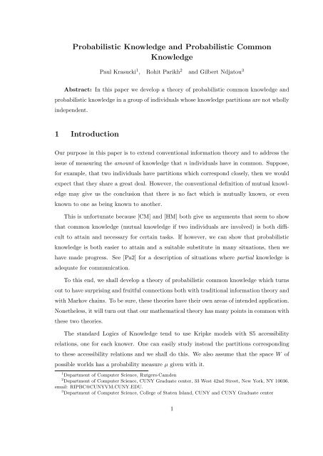
Probabilistic Knowledge and Probabilistic Common Knowledge 1 ...

Probabilistic Knowledge and Probabilistic Common
Knowledge
Paul Krasucki 1 , Rohit Parikh 2 and Gilbert Ndjatou 3
Abstract: In this paper we develop a theory of probabilistic common knowledge and
probabilistic knowledge in a group of individuals whose knowledge partitions are not wholly
independent.
1 Introduction
Our purpose in this paper is to extend conventional information theory and to address the
issue of measuring the amount of knowledge that n individuals have in common. Suppose,
for example, that two individuals have partitions which correspond closely, then we would
expect that they share a great deal. However, the conventional definition of mutual knowledge
may give us the conclusion that there is no fact which is mutually known, or even
known to one as being known to another.
This is unfortunate because [CM] and [HM] both give us arguments that seem to show
that common knowledge (mutual knowledge if two individuals are involved) is both difficult
to attain and necessary for certain tasks. If however, we can show that probabilistic
knowledge is both easier to attain and a suitable substitute in many situations, then we
have made progress. See [Pa2] for a description of situations where partial knowledge is
adequate for communication.
To this end, we shall develop a theory of probabilistic common knowledge which turns
out to have surprising and fruitful connections both with traditional information theory and
with Markov chains. To be sure, these theories have their own areas of intended application.
Nonetheless, it will turn out that our mathematical theory has many points in common with
these two theories.
The standard Logics of Knowledge tend to use Kripke models with S5 accessibility
relations, one for each knower. One can easily study instead the partitions corresponding
to these accessibility relations and we shall do this. We also assume that the space W of
possible worlds has a probability measure µ given with it.
1 Department of Computer Science, Rutgers-Camden
2 Department of Computer Science, CUNY Graduate center, 33 West 42nd Street, New York, NY 10036.
email: RIPBC@CUNYVM.CUNY.EDU.
3 Department of Computer Science, College of Staten Island, CUNY and CUNY Graduate center
1

In Figure I below, Ann has partition A = {A 1 , A 2 } and Bob has partition B = {B 1 , B 2 }
so that each of the sets A i , B j has probability .5 and the intersections A i ∩B j have probability
.45 when i = j and .05 otherwise.
The vertical line divides A 1 from A 2
The slanted line divides B 1 from B 2
.45
.05
▲
▲
▲
▲
▲
▲
.05 ▲
Figure I
.45
Since the meet of the partitions is trivial, there is no common knowledge in the usual
sense of [Au], [HM]. In fact there is no nontrivial proposition p such that Ann knows that
Bob knows p. It is clear, however, that Ann and Bob have nearly the same information
and if the partitions are themselves common knowledge, then Ann and Bob will be able to
guess, with high probability, what the other knows. We would like then to say that Ann and
Bob have probabilistic common knowledge, but how much? One purpose of this paper is to
answer this question and to prove properties of our definition that show why the answer is
plausible.
A closely related question is that of measuring indirect probabilistic knowledge. For
example, we would expect that what Ann knows about Bob’s knowledge is less than or
equal to what Bob himself knows, and what Ann knows of Bob’s knowledge of Carol is in
turn less than or equal to the amount of knowledge that Bob has about Carol’s knowledge.
We would expect in the limit that what Ann knows about what Bob knows about what
Ann knows... about what Bob knows will approach whatever ordinary common knowledge
they have.
It turns out that to tackle these questions successfully, we need a third notion. This
is the notion of the amount of information acquired when one’s probabilities change as a
result of new information (which does not invalidate old information). Suppose for example
that I am told that a certain fruit is a peach. I may then assign a probability of .45 to the
proposition that it is sweet. If I learn then that it just came off a tree, then I will expect
that it was probably picked for shipping and the probability may drop to .2, but if I learn
again that it fell off the tree, then it will rise to .9. In each case I am getting information,
consistent with previous information and causing me to revise my probabilities, but how
2

much information am I getting?
2 Preliminaries
We start by giving some definitions, some old, some apparently new. If a space has 2 n
points, all equally likely, then the amount of information gained by knowing the identity of
a specific point x is n bits. If one only knows a set X in which x falls, then the information
gained is less, in fact equal to I(X) = − log(µ(X)) where µ(X) is the probability 4 of X. If
P = P 1 , ..., P k is a partition of the whole space W , then the expected information when one
discovers the identity of the P i which contains x, is
k∑
k∑
H(P) = µ(P i )I(P i ) = −µ(P i ) log(µ(P i ))
i=1
i=1
These definitions so far are standard in the literature [Sh], [Ab], [Dr]. We now introduce
a notion which is apparently new.
Suppose I have a partition P = {P 1 , ..., P k } whose a priori probabilities are y 1 , ..., y k ,
but some information that I receive causes me to change them to u 1 , ..., u k . How much
information have I received?
Definition 1 :
k∑
k∑
IG(⃗u, ⃗y) = u i (log u i − log y i ) = u i log( u i
)
y
i=1
i=1 i
Here IG stands for “information gain”.
Clearly this definition needs some justification. We will first provide an intuitive explanation,
and then prove some properties of this notion IG which will make it more plausible
that it is the right one.
(a) Suppose that the space had 2 n points, and the distribution of probabilities that we
had was the flat distribution. Then the set P i has 2 n ·y i points 5 . After we receive our
information, the points are no longer equally likely, and each point in P i has probability
u i
|P i | = u i
y i 2 n . Thus the expected information of the partition of the 2 n singleton sets is
k∑
− (y i · 2 n ) u i
y
i=1
i 2 n log( u i
y i 2 n )
4 We will use the letter µ for both absolute and relative probabilities, to save the letter p for other uses.
All logs will be to base 2 and since x log(x) → 0 as x → 0 we will take x log(x) to be 0 when x is 0.
5 There is a tacit assumption here that the y i are of the form k/2 n . But note that numbers of this form
are dense in the unit interval and if we assume that the function IG is continuous, then it is sufficient to
consider numbers of this form.
3

which comes out to
k∑
α = n − u i (log u i − log y i )
i=1
Since the flat distribution had expected information n, we have gained information equal
to
k∑
k∑
k∑
n − α = n − (n − u i (log u i − log y i )) = u i (log u i − log y i ) = u i log( u i
)
y
i=1
i=1
i=1 i
(b) In information theory, we have a notion of the information that two partitions P and
Q share, also called their mutual information, and usually denoted by I(P; Q).
I(P; Q) = ∑ i,j
µ(P i ∩ Q j ) log( µ(P i ∩ Q j )
µ(P i ) · µ(Q j ) )
We will recalculate this quantity using the function IG. If Ann has partition P, then with
probability µ(P i ) she knows that P i is true. In that case, she will revise her probabilities
of Bob’s partition from µ( Q) ⃗ to µ( Q|P ⃗ i ) and and in that case her information gain about
Bob’s partition is IG(µ( Q|P ⃗ i ), µ( Q)). ⃗
Summing over all the P i we get
∑
µ(P i ) · IG(µ( Q|P ⃗ i ), µ( Q)) ⃗ = ∑
i
i
µ(P i )( ∑ j
(µ(Q j |P i ) log( µ(Q j|P i )
µ(Q j ) ))
and an easy calculation shows that this is the same as
I(P; Q) = ∑ i,j
µ(P i ∩ Q j ) log( µ(P i ∩ Q j )
µ(P i ) · µ(Q j ) )
Since the calculation through IG gives the same result as the usual formula, this gives
additional support to the claim that our formula for the information gain is the right one.
3 Properties of information gain
Theorem 1 : (a) IG(⃗u, ⃗v) ≥ 0 and IG(⃗u, ⃗v) = 0 iff ⃗u = ⃗v.
(b1) If ⃗p = µ(P ⃗ ) and if there is set X such that u i = µ(P i |X) for all i, then
IG(⃗u, ⃗p) ≤ −log(µ(X))
Thus the information received, by way of a change of probabilities, is less than or equal to
the information I(X) contained in X.
(b2) Equality obtains in (b1) above iff for all i, either µ(P i |X) = µ(P i ), or else µ(P i ∩X) = 0.
4

Thus if all nonempty sets involved have non-zero measure, every P i is either a subset of X
or disjoint from it.
Proof : (a) It is straightforward to show using elementary calculus that
log x < (x − 1) log e except when x = 1 when the two are equal. 6 Replacing x by 1/x we
get log x > (1 − 1/x) log e except again at x = 1. This yields
IG(⃗u, ⃗v) = ( ∑ i
u i (log u i
v i
)) ≥ ( ∑ i
u i (1 − v i
u i
)) log e = (( ∑ i
u i ) − ( ∑ i
v i )) log e = 0
with equality holding iff, for all i, either u i
v i
= 1, or u i = 0. However, the case u i = 0 cannot
arise, since we know that ∑ i u i = ∑ i v i = 1 and u i ≤ v i for all i.
(b1) Let u i = µ(P i |X), ⃗p = (µ(P 1 ), ..., µ(P k )).
IG(⃗u, ⃗p) =
k∑
i=1
k∑
i=1
µ(P i |X) log µ(P i|X)
µ(P i )
µ(P i |X) log µ(P i ∩ X)
µ(P i )
where α = ∑ k
i=1 µ(P i |X) log µ(P i∩X)
µ(P i )
=
k∑
i=1
µ(P i |X) log µ(P i ∩ X)
µ(P i )µ(X) =
k∑
− µ(P i |X) log µ(X)) = α + I(X)
i=1
≤ 0, since µ(P i∩X)
µ(P i )
≤ 1 for all i and ∑ k
i=1 µ(P i |X) = 1.
(b2) α = 0 only if, for all i, µ(P i |X) = 0 or µ(P i ∩ X) = µ(P i ), i.e. either P i ∩ X = ∅ or
P i ⊆ X (X is a union of the P i ’s).
If we learn that one of the sets can be excluded, that we had initially considered possible
(its probability was greater then zero), then our information gain is the least if the
probability of the excluded piece is distributed over all the other elements of the partition,
proportionately to their initial probabilities. the gain is greatest when the probability of the
excluded piece is shifted to a single element of the partition, and this element was initially
one of the least likely elements.
Theorem 2 : Let ⃗v = (v 1 , ..., v k−1 , v k ), ⃗u = (u 1 , ..., u k−1 , u k ), where u k = 0, u i =
v i + a i v k for i = 1, ..., k − 1, a i ≥ 0, ∑ k−1
i=1 a i = 1, and v k > 0. Then:
(a) IG(⃗u, ⃗v) is minimum when a i
v i
= c is the same for all i = 1, ..., k − 1, and c = 1
1−v k
.
moreover, this minimum value is just − log(1 − v k ).
(b) IG(⃗u, ⃗v) is maximum when a i = 1 for some i such that v i = min j=1...k−1 (v j ) and the
other a j are 0.
Proof : (a) Let a = (a 1 , ..., a k−2 , a k−1 ). Since ∑ k−1
i=1 a i = 1 we have a k−1 = 1− ∑ k−2
i=1 a i.
6 e is of course the number whose natural log is 1. Note that log e = log 2 e = 1 . The line y = (x−1) log e
ln 2
is tangent to the curve y = log x at (1,0), and lies above it.
✷
5

So we need only look at f : [0, 1] k−2 → R, defined by:
k−2
∑
f(⃗a) = IG(⃗u, ⃗v) = (v i +a i v k ) log v i + a i v k
i=1
k−2 ∑
+(v k−1 +v k (1−
v i
j=1
a j )) log (v k−1 + v k (1 − ∑ k−2
j=1 a j)
v k−1
To find the extrema of f in [0, 1] k−2 , consider the partial derivatives
∂f
∂a i
= 0 iff v i+a i v k
v i
for all i, a i
v i
= a k−1
v k−1
∂f
∂a i
= v k (log v i + a i v k
v i
= (v k−1+v k (1− ∑ k−2
v k−1
j=1 a j))
− log v k−1 + v k (1 − ∑ k−2
j=1 a j)
) log e
v k−1
. Recall that a k−1 = 1 − ∑ k−2
i=1 a i. Then we have
or a i = cv i where c is a constant and i range over 1, ..., k − 1. If we add
these equations and use the fact that ∑ k−1
i=1 a i = 1 and the fact that ∑ k−1
i=1 v i = 1 − v k we
get c = 1
1−v k
. Now ∂f
∂a i
is an increasing function of a i , so it is > 0 iff a i > v i
1−v k
and it is < 0
iff a i <
v i
1−v k
. Thus f has a minimum when a i =
v i
1−v k
for all i. The fact that this minimum
value is − log(1 − v k ) is easily calculated by substitution. Note that this quantity is exactly
equal to I(X) where X is the complement of the set P k whose probability was v k . Thus we
have an exact correspondence with parts (b1) and (b2) of the previous theorem.
(b) To get the maximum, note that since the first derivatives ∂f
∂a i
are always increasing,
and the second derivatives are all positive, the maxima can only occur at the vertices
of [0, 1] k−1 . (If they occurred elsewhere, we could increase the value by moving in some
direction). Now the values of f at the points p j = (0, ...0, 1, 0, ...0) (a i = δ(i, j)), are
IG(⃗u, ⃗v) = g(v j ) where g(x) = (x+v k ) log x+v k
x
. But g(x) = (x+v k) log x+v k
x
is a decreasing
function of x. so IG(u, v) is maximum when a j = 1 for some j such that v j is minimal. ✷
Example 1 : Suppose for example that a partition {P 1 , P 2 , P 3 , P 4 } is such that all the P i
have probabilities equal to .25. If we now receive the information that P 4 is impossible, then
we will have gained information approximately equal to IG(.33, .33, .33, 0, .25, .25, .25, .25) ≈
3·(.33) log .33
.25 ≈ log 4 3 ≈ .42. Similarly, if we discover instead that it is P 3 which is impossible.
If, however, we only discover that the total probability of the set P 3 ∪ P 4 has decreased to
.33, then our information gain is only IG(.33, .33, .17, .17, .25, .25, .25, .25) ≈ .08, which is
much less. And this makes sense, since knowing that the set P 3 ∪ P 4 has gone down in
weight tells us less than knowing that half of it is no longer to be considered, and moreover
which half.
If we discover that P 4 is impossible and all the cases that we had thought to be in P 4
are in fact in P 1 , then the information gain is IG(.50, .25, .25, 0, .25, .25, .25, .25) = 1 2 log 2
which is .5 and more than our information gain in the two previous cases.
6

Example 2 : As the following example shows, IG doesn’t satisfy the triangle inequality.
I.e. if we revise our probabilities form ⃗y to ⃗u and then again to ⃗v, our total gain can be
less than revising it straight from ⃗y to ⃗v. This may perhaps explain why we do not notice
gradual changes, but are struck by the cumulative effect of all of them.
Take ⃗v = (0.1, 0.9), ⃗u = (0.25, 0.75), ⃗y = (0.5, 0.5). IG(⃗v, ⃗u) + IG(⃗u, ⃗y) = 0.13 + 0.21 =
0.34, while IG(⃗v, ⃗y) = 0.53 (approximately). Also IG(⃗y, ⃗v) = 0.74 so that IG is not
symmetric.
Another way to see that this failure of the triangle equality is reasonable is to notice
that we could have gained information by first relativising to a set X, and then to another
set Y , gaining information ≤ − log(µ(X)) and − log(µ(Y )) respectively. However, to get
the cumulative information gain, we might need to relativise to X ∩ Y whose probability
might be much less than µ(X)µ(Y ).
We have defined the mutual knowledge I(P; Q) of two partitions P, Q. If we denote
their join as P +Q then the quantity usually denoted in the literature as H(P, Q)) is merely
H(P + Q). The connection between mutual information and entropy is well known [Ab]:
H(P + Q) = H(P) + H(Q) − I(P; Q)
Moreover, the equivocation H(P|Q) of P with respect to Q is defined as H(P|Q) = H(P) −
I(P; Q). If i and j are agents with respective partitions P i and P j respectively, then inf(ij)
will be just I(P i ; P j ).
The equivocations are non-negative, and I is symmetric, and so we have:
I(P; Q) ≤ min(H(P), H(Q))
Thus what Ann knows about Bob’s knowledge is always less than what Bob knows and
what Ann herself knows.
We want now to generalise these notions to more than two people, for which we will
need a notion from the theory of Markov chains, namely stochastic matrices. We start by
making a connection between boolean matrices and the usual notion of knowledge.
4 Common knowledge and Boolean matrices
We start by reviewing some notions from ordinary knowledge theory, [Au], [HM], [PK].
Definition 2 : Suppose that {1,...,k} are individuals and i has knowledge partition P i .
If w ∈ W then i knows E at w iff P i (w) ⊆ E, where P i (w) is the element of the partition
7

P i containing w. K i (E) = {w|i knows E at w}. Note that K i (E) is always a subset of E.
Write w ≈ i w ′ if w and w ′ are in the same element of the partition P i (iff P i (w) =
P i (w ′ )). Then i knows E at w iff for all w ′ , w ≈ i w ′ → w ′ ɛE.
Also, it follows that i knows that j knows E at w iff wɛK i (K j (E)) iff ⋃ l≤n {P j l|P j l ∩
P i (w) ≠ ∅} ⊆ E i.e. {w ′ |∃v such that w ≈ i v ≈ j w ′ } ⊆ E.
Definition 3 : An event E is common knowledge between a group of individuals
i 1 , ..., i m at w iff (∀j 1 , ..., j k ∈ {i 1 , ..., i m })(w ≈ j1 w 1 , ..., w k−1 ≈ jk w ′ ) → (w ′ ∈ E) iff for all
Xɛ{K 1 , ..., K n } ∗ wɛX(E).
We now analyse knowledge and common knowledge using boolean transition matrices 7 :
Definition 4 : The boolean transition matrix B ij of ij is defined by letting B ij (k, l) = 1
if P k
i
∩ P l j
≠ ∅, and 0 otherwise.
We can extend this definition to a string of individuals x = i 1 ...i k :
Definition 5 : The boolean transition matrix B x for a string x = i 1 ...i k is
B x = B i1 i 2
⊗ B i2 i 3
⊗ ... ⊗ B ik−1 i k
where ⊗ is defined as normalised matrix multiplication:
if (B × B ′ )(k, l) > 0 then (B ⊗ B ′ )(k, l) is set to 1, otherwise it is 0. We can also define ⊗
as: (B ⊗ B ′ )(k, l) = ∨ n
m=1 (B(k, m) ∧ B ′ (m, l))
We say that there is no non-trivial common knowledge iff the only event that is common
knowledge at any w is the whole space W .
Fact 1 : There is no non-trivial common knowledge iff for every string x including all
individuals, lim n→∞ B x n = 1 where 1 is the matrix filled with 1’s only.
We now consider the case of stochastic matrices.
5 Information via a string of agents
When we consider boolean transition matrices, we may lose some information. If we know
the probabilities of all the elements of the σ-field generated by the join of the partitions P i ,
the boolean transition matrix B ij is created by putting a 1 in position (k, l) iff µ(P l j |P k
i ) > 0,
and 0 otherwise. We keep more of the information by having µ(Pj l|P i k ) in position (k, l).
We denote this matrix by M ij and we call it the transition matrix from i to j.
7 The subscripts to the matrices will denote the knowers, and the row and column will be presented
explicitly as arguments. Thus B ij(k, l) is the entry in the kth row and jth column of the matrix B ij.
8

Definition 6 : For every i, j, the ij-transition matrix M ij is defined by: M ij (a, b) =
µ(P b j |P a
i ).
For all i, M ii is the unit matrix of dimension equal to the size of partition P i .
Definition 7 : If x is a string of elements of {1, ..., k} (x ∈ {1, ..., k} ∗ , x = x 1 ...x n ),
then M x = M x1 x 2
× ... × M xn−1 x n
is the transition matrix for x.
We now define inf(ixj), where x is a sequence of agents. inf(ixj) will be the information
that i has about j via x. If e.g. i = 3, x = 1, j = 2, we should interpret inf(ixj) as the
amount of information 3 has about 1’s knowledge of 2.
Example 3 : In our example in the introduction, If i were Ann and j were Bob, then
we would get
M ij =
∣
.9 .1
.1 .9
The matrix M ji equals the matrix M ij and the matrix M iji is
M iji =
∣
∣
.82 .18
.18 .82
Thus it turns out that each of Ann and Bob has .53 bits of knowledge about the other and
Ann has .32 bits of knowledge about Bob’s knowledge of her.
Definition 8 : Let ⃗m l = (m l1 , ..., m lk ) be the lth row vector of the transition matrix
M ixj (m lt = µ(Pj t| xPi l),
where µ(P j t| xPi l ) is the probability that a point in P
l
i will end up
in P t j
after a random move within P
l
i
within the elements of those P xr
∣
followed by a sequence of random moves respectively
which form x). Then:
k∑
inf(ixj) = µ(Pi l )IG( ⃗m l , µ(P ⃗ j ))
l=1
where IG( ⃗m l , µ(P ⃗ j )) is the information gain of the distribution ⃗m l over the distribution
µ(P ⃗ j ).
The intuitive idea is that the a priori probabilites of j’s partition are
⃗ µ(P j ). However,
if w is in Pi l , the l’th set in i’s partition, then these probabilities will be revised according
to the l’th row of the matrix M ixj and the information gain will be IG(⃗m l , µ(P ⃗ j )). The
expected information gain for i about j via x is then obtained by multiplying by the µ(P l
i )’s
and summing over all l.
Example 4 : Consider M iji . For convenience we’ll denote elements P m
i
elements P m j
by A m and
by B m (so that the A’s are elements of i’s partition, and the B’s are elements
9

of j’s partition). Therefore M iji = M ij × M ji where:
µ(B 1 |A 1 ) · · · µ(B k |A 1 )
µ(B 1 |A 2 ) · · · µ(B k |A 2 )
M ij =
. . .. M ji =
.
∣ µ(B 1 |A k ) · · · µ(B k |A k ) ∣ ∣
µ(A 1 |B 1 ) · · · µ(A k |B 1 )
µ(A 1 |B 2 ) · · · µ(A k |B 2 )
.
. .. .
µ(A 1 |B k ) · · · µ(A k |B k )
∣
M iji is the matrix of probabilities µ(A l | j A m ) for l, m = 1, ..., k, where µ(A l | j A m ) is the
probability that a point in A m , will end up in A l after a random move within A m followed
by a random move within some B s .
µ(A 1 | j A 1 ) µ(A 1 | j A 2 ) · · · µ(A 1 | j A k )
µ(A 2 | j A 1 ) µ(A 2 | j A 2 ) · · · µ(A 2 | j A k )
M iji =
. .
. .. .
∣ µ(A k | j A 1 ) µ(A k | j A 2 ) · · · µ(A k | j A k ) ∣
Note that for x = λ, where λ is the empty string, inf(ij) = I(P i ; P j ), as in the standard
definition: inf(ij) = ∑ k
l=1 µ(Pi l)IG(
µ(P
⃗ j |Pi l),
µ(P ⃗ j )) = ∑ k
l=1 µ(Pi l)
∑ k
t=1 µ(P j |Pi l)
log µ(P j t|P i l)
= ∑ k
l,t=1 µ(P j ∩ P l
i ) log µ(P t j ∩P l i )
µ(P t j )µ(P l i )
µ(P t j )
6 Properties of transition matrices
The results in this section are either from the theory of Markov chains, or easily derived
from these.
Definition 9 : A matrix M is stochastic if all elements of M are reals in [0,1] and the
sum of every row is 1.
Fact 2 : For every x, the matrix M x is stochastic.
Definition 10 : A matrix M is regular if there is m such that ∀(k, l)M m (k, l) > 0.
The following fact establishes a connection between regular stochastic matrices and
common knowledge:
Fact 3 :
individuals from x.
Matrix M ixi is regular iff there is no common knowledge between i and
Fact 4 : For every regular stochastic matrix M, there is a matrix M ′ such that
lim M n = M ′
n→∞
M ′ is stochastic, and all the rows in M ′ are the same. Moreover the rate of convergence is
exponential: for a given column r, let d n (r) be the difference between the maximum and
10

the minimum in M n , in that column. Then there is ɛ < 1 such that for all columns r and
all sufficiently large n, d n (r) ≤ ɛ n .
By combining the last two facts we get the following corollary:
Fact 5 : If there is no common knowledge between i and the individuals in x, then
lim (M ixi) n = M
n→∞
where M is stochastic, and all rows in M are equal to the vector ⃗u i of probabilities of the
sets in the partition P i .
A matrix with all rows equal represents the situation that all information is lost and all
that is known is the a priori probabilities.
Fact 6 : If L, S are stochastic matrices and all the rows of L are equal, then S × L = L,
and L × S = L ′ , where all rows in L ′ are equal (though they may be different from those of
L).
Fact 7 : For any stochastic matrix S and regular matrix M ixi :
S × lim
n→∞ (M ixi) n = M ′
where
M ′ = lim
n→∞ (M ixi) n
Definition 11 : For a given partition P i and string x = x 1 x 2 ...x k we can define a
relation ≈ x between the partitions P i and P j . P m
i ≈ x P n j iff for w ∈ P m
i and w ′ ∈ P n j ,
there are v 1 , ..., v k−1 such that v 1 ∈ P m
i , v k ∈ P n j and w ≈ x1 v 1 ≈ x2 ...v k−1 ≈ xk w ′ .
Definition 12 : ≈ ∗ x is the transitive closure of ≈ x . It is an equivalence relation.
Fact 8 : Assume that x contains all j. Then the relation ≈ ∗ x does not depend on the
particular x and we may drop the x. P m
i ≈ ∗ P n j iff P m
i and P n j are subsets of the same
element of P − where P − is the meet of the partitions of all the individuals.
Observation: We can permute the elements of the partition P i so that the elements of
the same equivalence class of ≈ ∗ have consecutive numbers and then M ixi looks as follows:
M ixi =
∣
∣
M 1 · · · 0 ∣∣∣∣∣∣
.
. .. .
0 · · · M r
where M l for l ≤ r is the matrix corresponding to the transitions within one equivalence
class of ≈ ∗ . All submatrices M l are square and regular.
11

Note that if there is no common knowledge then ≈ ∗ has a single equivalence class.
Since we can always renumber the elements of the partitions so that the transition matrix
is in the form described above, we will assume from now on that the transition matrix is
always given in such a form.
Fact 9 : If x contains all j then
lim (M ixi) n = M
n→∞
where M is stochastic, submatrices M l of M are regular (in fact positive) and all the rows
within every submatrix M l are the same.
7 Properties of inf(ixj)
Theorem 3 : If there is no common knowledge and x includes all the individuals, then
lim
n→∞ inf(i(jxj)n ) = 0
Proof : Matrix M = lim n→∞ (M jxj ) n has all rows positive and equal. Let ⃗m be a
row vector of M. Then lim n→∞ inf(i(jxj) n ) = IG(⃗m, µ(P ⃗ j )). Since the limiting vector ⃗m
is equal to the distribution µ(P ⃗ j ), we get: lim n→∞ inf(i(jxj) n ) = IG( µ(P ⃗ j ), µ(P ⃗ j )) = 0. ✷
The last theorem can be easily generalised to the following:
Fact 10 : If there is no common knowledge among the individuals in x, and i, j occur
in x, then as n → ∞, inf(ix n j) goes to zero.
8 Probabilistic common knowledge
Common knowledge is very rare. But, even if there is no common knowledge in the system,
we often have probabilistic common knowledge.
Definition 13 : Individuals {1, ..., n} have probabilistic common knowledge if
∀x ∈ {1, ..., n} ∗ inf(x) > 0
We note that there is no probabilistic common knowledge in the system iff there is some
string x such that for some i, M xi is a matrix with all rows equal and M xi (·, t) = µ(P t
i ) for
all t.
12

Theorem 4 : If there is common knowledge in the system then there is probabilistic
common knowledge, and
∀x ∈ {1, ..., n} ∗ inf(x) ≥ H(P − )
Proof
: We know from Fact 9 that
M ixi =
∣
∣
M 1 · · · 0 ∣∣∣∣∣∣
.
. .. .
0 · · · M r
where M l for l ≤ r is the matrix corresponding to the transitions within one equivalence class
of ≈ ∗ x, and all submatrices M l are square and regular. Here r is the number of partitions in
P − . Suppose that the probabilities of the sets in the partition P i are u 1 , ..., u k and that the
probabilities of the partition P − are w 1 , ..., w r . Each w j is going to be the sum of those u l
where the lth set in the partition P i is a subset of the jth set in the partition P − . Let ⃗m l
be the lth row of the matrix M ixi . Then inf(ixi) is ∑ k
l=1 u l IG(⃗m l , ⃗u). The row ⃗m l consists
of zeroes, except in places corresponding to subsets of the apppropriate element P − j of P − .
Then, by theorem 2, part (a): IG(⃗m i , ⃗u) ≥ log(
1
1−(1−w j ) ) = − log w j. This quantity
may repeat, since several elements of P i may be contained in P − j
. When we add up all the
multipliers u i that occur with log w j , these multipliers also add up to w j . Thus we get
r∑
inf(ixi) ≥ −w j log(w j ) = H(P − )
j=1
. ✷
We can also show:
Theorem 5 : If x contains i, j and there is common knowledge between i, j and all the
components of x, then the limiting information always exists and lim n→∞ inf(i(jxj) n ) =
H(P − )
We postpone the proof to the full paper.
References
[Ab] Abramson, N., Information Theory and Coding, McGraw-Hill, 1963
[AH] M. Abadi and J. Halpern, Decidability and expressiveness for first-order logics of probability,
Proc. of the 30th Annual Conference on Foundations of Computer Science, 1989,
pp. 148–153.
[Au] Aumann, R., “Agreeing to Disagree”, Annals of Statistics, 1976, 4, pp. 1236-1239
13

[Ba] F. Bacchus, On Probability Distributions over Possible Worlds, Proceedings of the 4th
Workshop on Uncertainty in AI, 1988, pp. 15-21
[CM] H. H. Clark and C. R. Marshall, “Definite Reference and Mutual Knowledge”, in
Elements of Discourse Understanding, Ed. Joshi, Webber and Sag, Cambridge U. Press,
1981.
[Dr] F. Dretske. Knowledge and the Flow of Information, MIT Press, 1981.
[Ha] J. Halpern, An analysis of first-order logics of probability, Proc. of the 11th International
Joint Conference on Artificial Intelligence (IJCAI 89), 1989, pp. 1375–1381.
[HM] Halpern, J. and Moses, Y., “Knowledge and Common Knowledge in a Distributed
Environment”, Proc. 3rd ACM Conf. on Principles of Distributed Computing, 1984, pp.
50-61
[KS] Kemeny, J. and Snell, L., Finite Markov Chains, Van Nostrand, 1960
[Pa] Parikh, R., “Levels of Knowledge in Distributed Computing”, Proc. IEEE Symposium
on Logic in Computer Science, 1986, pp. 322-331
[Pa2] Parikh, R., “A Utility Based Approach to Vague Predicates” To appear.
[PK] Parikh, R. and Krasucki, P. “Levels of Knowledge in Distributed Computing”, Research
report, Brooklyn College, CUNY (1986). Revised version of [Pa] above.
[Sh] Shannon, C., “Mathematical Theory of Communication” Bell System Technical Journal,
28, 1948. (Reprinted in: Shannon and Weaver, A Mathematical Theory of Communication
University of Illinois Press, 1964.)
14