Gernot Hoffmann Contents Gaussian Filters
Gernot Hoffmann Contents Gaussian Filters
Gernot Hoffmann Contents Gaussian Filters

Create successful ePaper yourself
Turn your PDF publications into a flip-book with our unique Google optimized e-Paper software.
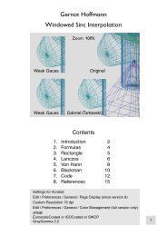
<strong>Gernot</strong> <strong>Hoffmann</strong><br />
<strong>Gaussian</strong> <strong>Filters</strong><br />
Carl Friedrich<br />
Gauß<br />
1777 - 1855<br />
<strong>Contents</strong><br />
1. Introduction 2<br />
2. Algorithm 3<br />
3. Blur Control 3<br />
4. Improvements 4<br />
5. Binary Weighting 5<br />
6. Arbitrary Filter Scaling 6<br />
7. Standard n-order Sharpening Filter 7<br />
8. General n-order Sharpening Filter 8<br />
9. Contour <strong>Filters</strong> 10<br />
10. Motion Blur 12<br />
11. Laplacian <strong>Filters</strong> 13<br />
12. Bode Plots for 2D <strong>Filters</strong> 17<br />
13. References 18<br />
Settings for Acrobat<br />
Edit / Preferences / General / Page Display (since version 6)<br />
Custom Resolution 72 dpi<br />
Edit / Preferences / General / Color Management (full version)<br />
sRGB<br />
EuroscaleCoated or ISOCoated or SWOP<br />
GrayGamma 2.2<br />
1
1. Introduction<br />
A <strong>Gaussian</strong> filter smoothes an image by calculating weighted averages in a filter box.<br />
Coordinates xo,yo are arbitrary pixel positions in a bitmap image. x,y is a local coordinate<br />
system, centered in xo,yo, as shown.<br />
The gray area is a filter box with m·m knots. Box coordinates x and y reach from -n to +n.<br />
The box width m=(2n+1) is assumed odd.<br />
Weight factors are calculated for a <strong>Gaussian</strong> bell by w(x,y)=e -a with a=(x 2 + y 2 )/(2r 2 ).<br />
The filter radius r is in statistics the standard deviation sigma.<br />
Choose n=(2...3)r or r=0.465n for a reasonable reproduction without clipping.<br />
E.g. for x=r, y=0 we find w= e -0.5 =0.6065.<br />
The image shows the function relative to the filter box vertically shifted. In the image the<br />
radius is r=2.<br />
The algorithm on page 2 is not optimized. The algorithm can be made much faster by binary<br />
weight factors, because then the whole calculation is in Integer and the multiplications are<br />
merely shifts (as on page 5).<br />
Note:<br />
The image quality is optimal only for direct view by Acrobat. Browsers are sometimes not<br />
accurate. Please use Zoom 100%.<br />
y<br />
x<br />
2
2. Algorithm<br />
General Weight Factors<br />
S=0<br />
r2=2·Sqr(r)<br />
For y=-n to +n Do<br />
For x=-n to +n Do<br />
Begin<br />
a=(Sqr(x)+Sqr(y))/r2<br />
w(x,y)=exp(-a)<br />
S=S+w(x,y)<br />
End<br />
3. Blur Control<br />
The blurring is controlled by two parameters:<br />
General Image Filtering<br />
1) The box width, described by m=(2n+1) pixels in one direction<br />
2) The radius r<br />
The <strong>Gaussian</strong> bell in one direction delivers:<br />
For yo=n to ymax-n Do<br />
For xo=n to xmax-n Do<br />
Begin<br />
newred=0<br />
newgrn=0<br />
newblu=0<br />
For y=-n to n Do<br />
For x=-n to n Do<br />
Begin<br />
newred=newred+w(x,y)·red(x+xo,y+yo)<br />
newgrn=newgrn+w(x,y)·grn(x+xo,y+yo)<br />
newblu=newblu+w(x,y)·blu(x+xo,y+yo)<br />
End<br />
newred=newred/S<br />
newgrn=newgrn/S<br />
newblu=newblu/S<br />
End<br />
x/r -3 -2 -1 0 1 2 3<br />
w(x) 0.0111 0.1353 0.6065 1.0 0.6065 0.1353 0.0111<br />
We can choose r=0.465n. This results in a weight factor 0.1 at the outermost pixel at x=n,<br />
which seems to be reasonable. Less than 0.1 does not make much sense. For pixels on the<br />
diagonal corners of the xy-box the value is anyway smaller.<br />
Weight factors. Weak blur n=1, r=0.465. Strong blur n=3, r=1.398.<br />
Weak blur: 0.100 1.0 0.100<br />
Strong blur: 0.100 0.358 0.773 1.0 0.773 0.358 0.100<br />
3
4. Improvements<br />
The Gauss formula can be separated. This will make the calculations faster.<br />
w(x,y) = e -(xx+yy) = w(x)w(y) = e -xx ·e -yy<br />
Another method uses one source image, one array of the same size for the accumulation and<br />
a sequence of shifted images. This shifted image is made once for each position x,y for all<br />
pixels in the source image.<br />
The author prefers the standard structure, because this is valid for any linear filter, like softening<br />
(blurring), sharpening and contour finding filters, also for some effects which use<br />
oscillations in the box.<br />
A 5x5 binary <strong>Gaussian</strong> filter, programmed mainly in Intel Assembly Language, needs about<br />
one second for 1000x1000 pixels (PC 400MHz).<br />
Note: the <strong>Gaussian</strong> filter in the straightforward kernel implementation cannot be executed<br />
inplace. One needs always a source framebuffer and a destination framebuffer.<br />
4
5.1 Binary Weighting<br />
This filter shows a crude approximation of the<br />
<strong>Gaussian</strong> bell function.<br />
The weight factors are powers of 2, thus multiplications<br />
by weight factors can be replaced<br />
by binary shifting.<br />
The sum of the weight factors is S=80. If all<br />
colors values are 255, then the weighted sum<br />
is 20400, which does not exceed the positive<br />
number space for Integer 2 15 -1=32767.<br />
Radius r=0.85, approximately.<br />
0 1 2 1 0<br />
1 4 8 4 1<br />
2 8 16 8 2<br />
1 4 8 4 1<br />
0 1 2 1 0<br />
For more general applications binary weighting by LongInt (32bit) could be used. This is still<br />
much faster than floating point operations.<br />
Part of a digital photo. Left not filtered. Right softened by Binary Weight Filter. Then both<br />
images were scaled down for 50 % and placed into PDF by pixel synchronization.<br />
The synchronization is perfect only for direct view by Acrobat but not necessarily by browser.<br />
5
5.2 Binary Weighting Transfer Function<br />
Gain transfer function for Binary Gauss 2-8-16-8-2<br />
6. Arbitrary Filter Scaling<br />
If the weight factors belong to a consistent set of<br />
data, like in the previously mentioned softening filters,<br />
then we have to divide all raw weight factors by the<br />
sum of the raw weight factors.<br />
Not so for a general sharpening filter.<br />
We start by a positive peak in the center and all negative<br />
values are taken from a <strong>Gaussian</strong> bell.<br />
The binary weighting is not essential in this example.<br />
Generally spoken, we have raw positive weight factors<br />
P i and raw negative weight factors N i .<br />
The actual filtering is done by scaled weight factors<br />
p i =2P i / S p and n i =N i / S n .<br />
S p = Sum of positive weight factors P i<br />
S n = Sum of negative weight factors |N i |<br />
-0 -1 -2 -1 -0<br />
-1 -4 -8 -4 -1<br />
-2 -8 +64 -8 -2<br />
-1 -4 -8 -4 -1<br />
-0 -1 -2 -1 -0<br />
This scaling is based on the demand that a uniform color area should deliver the same color<br />
after filtering.<br />
Example, as above:<br />
Sp = 64<br />
Sn = 4·8 + 4·4 + 4·2 + 8·1 = 64<br />
The center peak in the scaled matrix is +2 and the other negative values are divided by 64.<br />
For band pass and highpass filters we use equal sums and a contrast factor:<br />
p i =CP i / S p and n i =CN i / S n .<br />
6
7. Standard n-order Sharpening Filter<br />
1 2 3 4 5<br />
6 7 8 9 10<br />
11 12 13 14 15<br />
16 17 18 19 20<br />
21 22 23 24 25<br />
-0.0035 -0.0159 -0.0262 -0.0159 -0.0035<br />
-0.0159 -0.0712 -0.1173 -0.0712 -0.0159<br />
-0.0262 -0.1173 2.0 -0.1173 -0.0262<br />
-0.0159 -0.0712 -0.1173 -0.0712 -0.0159<br />
-0.0035 -0.0159 -0.0262 -0.0159 -0.0035<br />
The drawing shows the numbering and the weight factors for the kernel for a sharpening filter,<br />
here with n=2. The algorithm works for any n ≥1. The total number of elements is N=(2n+1) 2 .<br />
The center weight factor fs[13]=2.0 is a positive peak. The other weight factors fs[k] are<br />
calculated by a negative <strong>Gaussian</strong> bell, according to the code below.<br />
The sum of negative weight factors is -1.0 and the sum of all weight factors is +1, therefore a<br />
uniformly colored area remains unfiltered, as required.<br />
Tutorial code, not optimized<br />
sm:=0;<br />
k :=1;<br />
For j:=-n to n Do<br />
For i:=-n to n Do<br />
Begin<br />
ra:=Sqrt(Sqr(i)+Sqr(j))/n;<br />
ra:=exp(-2*Sqr(ra));<br />
fs[k]:=-ra;<br />
If (i0) Or (j0) Then sm:=sm+ra;<br />
Inc(k);<br />
End;<br />
k :=1;<br />
For j:=-n to n Do<br />
For i:=-n to n Do<br />
Begin<br />
fs[k]:=fs[k]/sm;<br />
If (i=0) And (j=0) Then fs[k]:=2.0;<br />
Inc(k);<br />
End;<br />
7
8.1 General n-order Sharpening Filter / Konzept<br />
This drawing shows the signal flow for a general sharpening filter. The low-pass filter Fn can<br />
be established by a <strong>Gaussian</strong> bell as explained in the chapters 1 to 3.<br />
K-1<br />
Low-pass<br />
filter Fn<br />
-<br />
C K<br />
D<br />
+<br />
The input C is an unfiltered value C=R,G or B at the center positition. The output D is the<br />
sharpened value at the same center position. The low-pass filter executes the averaging as<br />
usual by a <strong>Gaussian</strong> bell. The filtered value is subtracted from the unfiltered value, but the two<br />
are muliplied by factors (K-1) and K.<br />
D = [ K - (K-1) Fn ] C<br />
The factor K has this meaning:<br />
K=1 no sharpening<br />
K=2 sharpening as in previous chapter<br />
K=1.5 less sharpening than for K=2<br />
K=2 is a very reasonable value but sometimes a little more control for the filtering is<br />
welcome.This filter has two degrees of freedom: the filtering order n and the factor K.<br />
For a uniformly colored area the low-pass filter delivers just the input C and the total output D<br />
is the unchanged input C as well.<br />
Note: the sharpening filter as above and the blurring filter (low-pass) are not complementary.<br />
This means that sequential applications do not cancel each other.<br />
8
8.2 General n-order Sharpening Filter / Example<br />
Example: a weak sharpening filter with n=1 and K=1.5. Mainly for eyes and hair in portraits.<br />
0 0 0<br />
K −1<br />
F = K 0 1 0 −<br />
0 0 0 25 .<br />
18 / 14 / 18 /<br />
14 / 1 14 /<br />
18 / 14 / 18 /<br />
The upper diagram shows the Bode plot for the low pass filter. The lower diagram shows the<br />
Bode plot for the sharpening filter. Coefficients were re-calculated according to chapter 12.<br />
Use in PDF<br />
72 dpi / zoom 200%<br />
9
9.1 Contour <strong>Filters</strong> / Concept<br />
The well-known contour filters by Sobel, Roberts and Prewitt [3] use 3x3 kernels, which have<br />
to be applied twice: in x- and y-direction.<br />
They can be easily substituted by the nonlinear filter below, which finds contours in one pass.<br />
The sum of the absolute values of pixel differences in four directions is compared with an<br />
adjustable threshold.<br />
The example works for gray images. The actual implementation calculates contributions of<br />
three channels RGB and is programmed entirely in assembly code.<br />
The contour filter creates a black-on-white mask, which is normally hidden. At black points,<br />
the original photo can be blurred (anti-aliasing) or sharpened (enhanced edges).<br />
The famous Canny Edge filter is based on a multi-pass approach. Opposed to the filters<br />
above, the contour is delivered by single pixel lines or fragments of them.<br />
Procedure FContour(xa,ya,xe,ye: Integer; thresh: Single);<br />
{ Uses 3x3 points in area xa..xe, xa..ye }<br />
{ 1 2 3<br />
4 5 6<br />
7 8 9 }<br />
Var cc,clim : Single;<br />
x,y,c1,c2,c3,c4,c6,c7,c8,c9 : Integer; { 16 bit }<br />
prgb1,prgb2,prgb3,prgb4,prgb6,prgb7,prgb8,prgb9: LongInt; { 32 bit }<br />
Begin<br />
clim:=50+250*(thresh-0.1); { Threshold 0...1 }<br />
FMemGrYIQ (xa,ya,xe,ye,xa,ya,2); { FMem gray }<br />
FMemtoPMem (xa,ya,xe,ye,xa,ya); { PMem copy }<br />
ColToSx (0,0,gmx,gmy,stan,whit); { Screen white, global gmx,gmy }<br />
For y:=ya+1 To ye-1 Do<br />
Begin<br />
For x:=xa+1 To xe-1 Do<br />
Begin<br />
prgb1:=GetPixel (x-1,y-1); { PMem }<br />
prgb2:=GetPixel (x ,y-1);<br />
prgb3:=GetPixel (x+1,y-1);<br />
prgb4:=GetPixel (x-1,y );<br />
prgb6:=GetPixel (x+1,y );<br />
prgb7:=GetPixel (x-1,y+1);<br />
prgb8:=GetPixel (x ,y+1);<br />
prgb9:=GetPixel (x+1,y+1);<br />
c1:=prgb1 AND $000000FF;<br />
c2:=prgb2 AND $000000FF;<br />
c3:=prgb3 AND $000000FF;<br />
c4:=prgb4 AND $000000FF;<br />
c6:=prgb6 AND $000000FF;<br />
c7:=prgb7 AND $000000FF;<br />
c8:=prgb8 AND $000000FF;<br />
c9:=prgb9 AND $000000FF;<br />
cc:=Abs(c1-c9)+Abs(c2-c8)+Abs(c3-c7)+Abs(c4-c6);<br />
If cc>clim Then SetSixel(x,y,0); { Screen black }<br />
End; { x }<br />
End; { y }<br />
End;<br />
10
9.2 Contour <strong>Filters</strong> / Examples<br />
Use in PDF<br />
72 dpi / zoom 200%<br />
Threshold 0.5<br />
11
10.1 Motion Blur / Concept / Example 45°<br />
Motion blur can be created by an elliptic <strong>Gaussian</strong> bell. The longer axis ‘a’ is aligned with the<br />
velocity vector. The elliptic <strong>Gaussian</strong> bell is created in coordinates u,v for an axis aligned<br />
ellipse and then transformed into a rotated ellipse in x,y.<br />
The filter box contains many zeros and values near to zero. The speed can be increased by<br />
rounding near-zeros to zero and not executing filtering for these weight factors. A more tricky<br />
solution could use a list of valid weight factors.<br />
The effect is very similar to motion blur by Photoshop®.<br />
Va:=intens; { Velocity 0...2 }<br />
n:=Round(10*Va);<br />
If n
11.1 Laplacian <strong>Filters</strong> / Concept / Preliminary<br />
Laplacian filters are used e.g. in the context of the Canny Edge algorithm.<br />
A general Laplacian filter is derived from a <strong>Gaussian</strong> bell as the sum of the second derivatives<br />
(Laplacian of <strong>Gaussian</strong>, LoG):<br />
2 2<br />
x + y<br />
−<br />
2<br />
2σ<br />
fxy (,) = e<br />
wxy (,) = f + f<br />
xx yy<br />
2 2<br />
x + y<br />
−<br />
2<br />
2σ<br />
= e ( −1)<br />
w(,)<br />
xy = e ( −r)<br />
2<br />
σ<br />
2<br />
-r<br />
2 1 2<br />
2 2<br />
x + y<br />
2 σ<br />
2<br />
For convenience, the leading factor was ignored and the sign reversed.<br />
For cross sections of the functions f(x,y) and w(x,y) in one direction, we can set y= 0. This is<br />
not the same as drawing the functions for the bell f(x) and w(x). Here we would have w(σ)= 0.<br />
For the function w(x,y) we have w(σ,σ)=0.<br />
The graphic shows the bell (red), the Laplacian filter gain in one direction (green) and an<br />
equivalent Damped Cosine (blue), which is a kind of Gabor filter.<br />
Tic marks are in sigma-distance.<br />
For a sufficiently large kernel and properly normalized, this filter will work blurring with edge<br />
enhancement. This is agreeable for noisy images.<br />
Opposed to the design as above, the simplest Laplacian filter for edge detection is a high pass<br />
filter (here with reversed sign, compared to text books, which does not matter):<br />
⎡ 0 −1<br />
0⎤<br />
⎢−<br />
1 + 4 −1⎥<br />
⎣<br />
⎢ 0 −1<br />
0⎦<br />
⎥<br />
The LoG filter and the Damped Cosine filter can be converted into true band pass filters (high<br />
pass for smallest kernel) by a special normalization:<br />
Sum of positive values equal to +1, sum of negative values equal to -1.<br />
The following examples are valid for this normalization.<br />
13
11.2 Laplacian <strong>Filters</strong> / Band Pass / Code<br />
This code was tested:<br />
n:=Round(radius);<br />
If n16 Then n:=16;<br />
sig:=0.465*n; s2:=2*Sqr(sig);<br />
k:=1; fp:=0; fm:=0; Pfil:=2;<br />
Case PFil Of<br />
1: Begin<br />
For y:=-n to n Do<br />
For x:=-n to n do<br />
Begin<br />
r2:=(Sqr(x)+Sqr(y))/s2;<br />
fsk:=exp(-r2)*(r2-1);<br />
If fsk>0 Then fp:=fp+fsk Else fm:=fm-fsk;<br />
fs[k]:=fsk;<br />
Inc(k);<br />
End;<br />
End;<br />
2: Begin<br />
For y:=-n to n Do<br />
For x:=-n to n do<br />
Begin<br />
r2:=Sqr(x)+Sqr(y);<br />
r1:=1.25*pi*Sqrt(r2)/n;<br />
r2:=r2/s2;<br />
fsk:=exp(-r2)*cos(r1);<br />
If fsk>0 Then fp:=fp+fsk Else fm:=fm-fsk;<br />
fs[k]:=fsk;<br />
Inc(k);<br />
End;<br />
End;<br />
{ Alternatives for simple filters }<br />
3: Begin<br />
n:=1;<br />
fs[1]:=-0.5; fs[2]:=-1; fs[3]:=-0.5;<br />
fs[4]:=-1; fs[5]:=+8; fs[6]:=-1;<br />
fs[7]:=-0.5; fs[8]:=-1; fs[9]:=-0.5;<br />
fp:=8;<br />
fm:=6;<br />
End;<br />
4: As on previous page<br />
{ Contrast=0..10 }<br />
k:=1;<br />
For y:=-n to n do<br />
For x:=-n to n do<br />
Begin<br />
fsk:=fs[k];<br />
If fsk>0 Then fs[k]:=contr*fsk/fp Else fs[k]:=contr*fsk/fm;<br />
Inc(k);<br />
End;<br />
14
11.3 Laplacian <strong>Filters</strong> / Band Pass / Bode Plots<br />
Bode plots for normalized<br />
band pass filters for n=8<br />
Use in PDF<br />
72 dpi / zoom 200%<br />
Laplacian band pass filter<br />
Damped Cosine<br />
Better results for images<br />
Optimized filter<br />
This delivers bad results<br />
for images (double lines)<br />
15
11.4 Laplacian <strong>Filters</strong> / Band Pass / Examples<br />
Application of bandpass filters for n=8, contrast=2<br />
and background gray 128.<br />
Noise can be removed by tri-level posterization.<br />
Bottom left: Laplacian band pass<br />
Bottom right: Damped Cosine band pass<br />
16
12. Bode Plots for 2D <strong>Filters</strong><br />
<strong>Filters</strong> with weight factors w(x,y) are called 2D filters. Bode plots are shown for 1D weight<br />
factors w(x).<br />
The 2D filters have (mostly) radial symmetry, but it is not correct to use just the center row<br />
values as weight factors w(x) for the Bode plots.<br />
An image may consist of a left dark gray half and a right light gray half. It has a vertical edge.<br />
Obviously it is possible to achieve by a one-row filter w(x) the same effect as using the 2D filter<br />
- the edge can be blurred or sharpened.<br />
The 1D filter w(x) consists of the sum of the weight factors w(x,yi ) in each column of the 2D<br />
filter.<br />
The one-row filter w(x) is normalized as described in chapter 6.<br />
For low pass filters:<br />
Sum of positive factors: +2<br />
Sum of negative factors: -1<br />
For band pass and high pass filters (eventually using a contrast factor):<br />
Sum of positive factors: +1<br />
Sum of negative factors: -1<br />
Example for a Laplacian band pass:<br />
n:=8;<br />
sig:=0.465*n;<br />
s2 :=2*Sqr(sig);<br />
For x:=-n to n do<br />
Begin<br />
fsx:=0;<br />
For y:=-n to n do<br />
Begin<br />
r2 :=(Sqr(x)+Sqr(y))/s2;<br />
fsx:=fsx+exp(-r2)*(1-r2);<br />
End;<br />
fs[x]:=fsx;<br />
End;<br />
fp:=0; fm:=0;<br />
For x:=-n to n do<br />
Begin<br />
fsx:=fs[x];<br />
If fsx>0 Then fp:=fp+fsx Else fm:=fm-fsx;<br />
End;<br />
For x:=-n to n do<br />
Begin<br />
fsx:=fs[x];<br />
If fsx>0 Then fs[x]:=fsx/fp Else fs[x]:=fsx/fm;<br />
End;<br />
17
13. References<br />
[1] Elmar Schrüfer<br />
Signalverarbeitung<br />
Carl Hanser Verlag, München,Wien 1990<br />
[2] Samuel D.Stearns<br />
Digitale Verarbeitung analoger Signale<br />
R.Oldenbourg Verlag, München Wien 1988<br />
[3] Carsten Köhn<br />
Bildanalyse und Bilddatenkompression<br />
Carl Hanser Verlag München Wien 1996<br />
[4] <strong>Gernot</strong> <strong>Hoffmann</strong><br />
Fast Fourier Transform / Descreening<br />
http://www.fho-emden.de/~hoffmann/fft31052003.pdf<br />
Web docs about the filters will be added later.<br />
This doc<br />
http://www.fho-emden.de/~hoffmann/gauss25092001.pdf<br />
<strong>Gernot</strong> <strong>Hoffmann</strong><br />
September 30 / 2006<br />
Website<br />
Load browser / Click here<br />
18


![[PDF] SpieleProgrammierung](https://img.yumpu.com/6860251/1/190x135/pdf-spieleprogrammierung.jpg?quality=85)