2D Momentum Conservation - Saddleback College
2D Momentum Conservation - Saddleback College
2D Momentum Conservation - Saddleback College

Create successful ePaper yourself
Turn your PDF publications into a flip-book with our unique Google optimized e-Paper software.
2-D <strong>Momentum</strong> <strong>Conservation</strong><br />
<strong>Saddleback</strong> <strong>College</strong> Physics Department<br />
Purpose: To confirm that linear momentum is conserved in two-dimensional collisions. To<br />
show that kinetic energy is nearly conserved in two-dimensional near-elastic collisions.<br />
Equipment:<br />
collision ramp<br />
2 steel balls about 1 cm in diameter (with approximately the same mass)<br />
plumb line<br />
meter stick<br />
2 sheets of paper for each lab partner, about 70 cm square<br />
2 pieces of carbon paper<br />
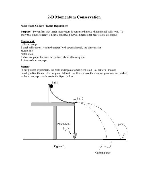
Sketch:<br />
In our present experiment, the balls undergo a glancing collision (i.e. center of masses<br />
misaligned) at the end of a ramp and fall onto the floor, where their impact positions are marked<br />
with carbon paper as shown in the figure below.<br />
Ball 1<br />
Ball 2<br />
Plumb bob<br />
paper<br />
Figure 2.<br />
Carbon paper
Theory:<br />
CONSERVATION OF MOMENTUM<br />
In any collision, with no net external forces acting on the system, linear momentum is<br />
conserved. A typical case is shown in the figure below, where the incoming ball, 1, undergoes a<br />
glancing collision with a target ball, which is initially at rest. After the collision, both balls<br />
move off at an angle to the original path of ball 1. Note that = 0 and therefore is not shown<br />
in figure 1 below.<br />
P 2 o<br />
ball 1<br />
ball 1<br />
P 1 f<br />
P 10<br />
P 1 0<br />
ball 2<br />
P 2 f<br />
P 2 f<br />
P 1 f<br />
+y<br />
+x<br />
Figure 1.<br />
v v<br />
P1<br />
+ P2<br />
f<br />
f<br />
Note that the vector sum of the final momenta is equal to the initial momentum. In the example<br />
drawn above, the collision occurs in a plane although the method could be used to analyze a<br />
similar three-dimensional collision. Applying conservation of linear momentum to the situation<br />
described above, using the shown coordinate system, yields:<br />
Px<br />
1 0<br />
Px<br />
1<br />
+ Px<br />
2<br />
= ⇒<br />
f<br />
f<br />
m1 vx<br />
1<br />
= m1v<br />
x1<br />
+ m2vx2<br />
o<br />
(1)<br />
f<br />
f<br />
Py<br />
1 0<br />
Py<br />
1<br />
+ Py<br />
2<br />
= ⇒<br />
f<br />
f<br />
m1 v<br />
y1<br />
= m1v<br />
y1<br />
+ m v<br />
o<br />
f 2 y2<br />
where P<br />
x<br />
and P<br />
y<br />
represent the corresponding x and y components of momentum. The<br />
subscripts o and f represent initial (i.e. before the collision) and final (i.e. after the collision)<br />
respectively, and ball 1 is the incoming ball while ball 2 is the target.<br />
f<br />
(2)<br />
As both of the balls fall at the same rate and strike the paper at the same time, the horizontal<br />
distance they move (their range) will be proportional to the velocity of the balls in the plane of<br />
the floor. Multiplying this distance by the mass of each ball will yield a number proportional to<br />
the momentum.<br />
If the masses are equal ( m 1<br />
= m 2<br />
= m ) then equations (1) & (2) become<br />
vx<br />
1<br />
= vx<br />
1<br />
+ v<br />
f x2<br />
f<br />
o<br />
(3)<br />
v<br />
y1 = v<br />
y1<br />
+ v<br />
o<br />
f y2<br />
f<br />
(4)
Since there is no acceleration in the horizontal plane ∆ x = vt and ∆ x = d , where d = distance.<br />
Solving for v gives<br />
d<br />
v = (5)<br />
t<br />
Substituting equation (5) into equations (3) & (4)<br />
d d<br />
1o<br />
x1<br />
f<br />
=<br />
t t<br />
d<br />
x<br />
+<br />
t<br />
x 2 f<br />
d d d<br />
y1o<br />
y1<br />
f y2<br />
f<br />
= +<br />
t t t<br />
Realizing the balls all take the same time, t, to fall yields<br />
d<br />
x1 = d<br />
x1<br />
+ d<br />
o x2<br />
(6)<br />
d<br />
y1 = d<br />
y1<br />
+ d<br />
o<br />
f y2<br />
f<br />
f<br />
or<br />
d1 = d1<br />
+ d<br />
f 2 f<br />
o<br />
(8)<br />
f<br />
(7)<br />
CONSERVATION OF KINETIC ENERGY<br />
If the collision is perfectly elastic, then the kinetic energy, K, of the system is also conserved.<br />
K1 = K1<br />
f<br />
+ K<br />
2 f<br />
o<br />
(9)<br />
or<br />
1<br />
2<br />
1 1<br />
m<br />
o<br />
+ (10)<br />
2<br />
2<br />
2<br />
1v<br />
= m 1 1v<br />
f1<br />
2 m2v f 2<br />
2<br />
If the masses are equal ( m 1<br />
= m 2<br />
= m ) equation (10) becomes<br />
2 2 2<br />
1<br />
= v1<br />
f<br />
v2<br />
f<br />
v + (11)<br />
o<br />
Using the same reasoning as for momentum conservation above, equation (11) becomes<br />
2 2 2<br />
1<br />
= d1<br />
f<br />
d<br />
2 f<br />
d<br />
o<br />
+ (12)<br />
Procedure:<br />
(a) Initial Set-Up<br />
1. The collision ramp should be securely fastened to the edge of the lab table. Adjust the target<br />
ball (ball 2) support so that the centers of both balls lie in a horizontal plane when they<br />
collide ( a 2-D collision is desired, not a 3-D collision).<br />
2. Align the plumb line so that it hangs directly below the point of collision. Tape the paper<br />
(no carbon paper yet) to the floor so that it is positioned as shown in figure 2. And mark the<br />
position of the plumb bob on the paper.<br />
3. Place the target ball (ball 2) on its support. Place the second ball on the ramp at the 10-cm<br />
mark and release it. Note approximately where the two balls strike the paper. If either ball
misses the paper, change the angular adjustment of the target support until both strike in a<br />
satisfactory position.<br />
4. Remove the target ball (ball 2) from its support and allow the incident ball (ball 1) to leave<br />
the edge of the ramp without a collision (still release it from the 10-cm mark!); it should<br />
also strike the paper. If it does not, either move the paper (and make a new plumb line<br />
mark) or release ball 1 from a lower point on the ramp. Make sure that the incident ball<br />
(ball 1) does not strike the target ball support screw as it leaves the ramp.<br />
(b) Taking Data<br />
1. Place a piece of carbon paper face down in the approximate position that the ball 1 struck<br />
the paper in part 4 above. Try to adjust the position of the carbon paper so that secondary<br />
bounces of the ball will not leave marks. Release the ball from the 10-cm mark on the ramp<br />
5 times, checking between trials to see that clear marks are being left under the carbon<br />
paper.<br />
2. Place the target ball (ball 2) on it’s support and release ball 1 from the 10 cm mark,<br />
observing the approximate position of where the two balls strike the paper. Place a sheet of<br />
carbon paper at the position of each strike, again being careful to place the carbon paper so<br />
that secondary bounces will not leave marks.<br />
3. Record the strike position of the two balls on the paper for 5 collisions. If the strike points<br />
on the paper are reasonably well clustered (say no more than a few cm spread) remove the<br />
paper (replacing it with a new piece) and repeat steps 1 – 3 of procedure (b) until each lab<br />
partner has a complete data sheet. Be sure to mark the position of the plumb line (your<br />
origin) on each data sheet and draw a set of axes with one axis parallel to the collision ramp!<br />
4. Change the angular position of the target ball, ball 2, and repeat the entire procedure (b). If<br />
it is necessary to release ball 1 from a different point on the track, when changing the<br />
angular position for ball 2, be sure to release ball 1 from this same point for all data runs<br />
done during this second half of the experiment.<br />
5. Before leaving the lab, obtain the instructor’s signature on your data sheets. Each lab<br />
partner should have 2 different completed data sheets with 5 sets of data on each.<br />
Analysis:<br />
(a)<br />
On each data sheet make a careful construction of the vector sum using the<br />
parallelogram method, like that shown below.<br />
plumb mark<br />
P 2 f<br />
P 1f<br />
v<br />
+<br />
v<br />
P1<br />
P<br />
f 2 f
You will have to estimate the middle of each cluster, ignoring any points that are obviously in<br />
error. Secondary bounce marks can usually be distinguished because they are noticeably lighter<br />
than true data points.<br />
In your conclusion give the percent difference between the magnitude of the initial<br />
momentum vector P v v v<br />
1<br />
and the vector sum of the final momenta ( P P<br />
0<br />
1f<br />
+<br />
2 f<br />
), use the average of<br />
P v v v<br />
1 0<br />
and ( P1<br />
P<br />
f<br />
+<br />
2 f<br />
) in the denominator of the percent difference equation. As percent difference<br />
is dimensionless, you can work in arbitrary momentum units, such as the distances measured on<br />
the data page. In your conclusion you should also give the angular difference between P v<br />
1<br />
and<br />
0<br />
v v<br />
+ . Repeat the above calculations for your second data sheet.<br />
P1<br />
P<br />
f 2 f<br />
(b)<br />
Measure the magnitude of each displacement vector, d, on the data pages and use<br />
equation (12)<br />
2 2 2<br />
d<br />
1o = d1<br />
f<br />
+ d<br />
2 f<br />
(12)<br />
where the d’s are the distances measured directly on the data sheets. In your conclusion, give<br />
the percent difference between the left-hand and right-hand sides of eqn (12) [where the<br />
denominator is the average of the left and right sides of eqn (12)].<br />
Elementary Error Propagation: (Note: This does not fulfill your error propagation<br />
requirements!) Estimate the uncertainty in d, δ d , taking into account the difficulty in<br />
estimating the middle of each cluster. Compare this uncertainty to the difference between<br />
and<br />
2 2<br />
1 f<br />
d<br />
2 f<br />
d + . Repeat for your second data sheet. It is not necessary to estimate the random<br />
error or uncertainty for the angle measurements. You decide if your experiment is successful<br />
based upon whether δ d is greater than, less than or equal to<br />
2 2 2<br />
( d1 f<br />
d<br />
2 f<br />
) − d1<br />
o<br />
+ .<br />
2<br />
d<br />
1o