real-time mbs formulations: towards virtual engineering

176 J. Cuadrado, M. Gonzalez, R. Gutierrez, M.A. Naya
3.2 Serial robot
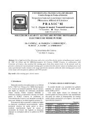
The PUMA robot, designed by Unimation & Co. and shown in Figure 3, is an example of a 6
degrees-of-freedom serial manipulator. It has been often used by different authors [9] to illustrate
methods and procedures in several areas of robotics. In this work, the robot has been taken as an
example of multibody system undergoing changing configurations.
Starting from rest, torques at the six hinges of the robot are provided so that, in a time of 2 s, it
arrives at a new position in the space, again in rest conditions. Once
the new position has been reached, a point of the hand is attached to
the ground, so that the robot loses 3 degrees-of-freedom. In this
new configuration, torques are applied to the three rotational pairs
of the hand, and a second maneuver, which lasts 4 s and ends with
rest conditions, is performed. Finally, the robot is released from its
attachment and returned in 2 s to the initial position by torques
acting at the six revolute joints, once more finishing the maneuver
at rest conditions. Therefore, the total simulation time is 8 s.
Table 2 illustrates the results obtained when applying the
proposed method. The error has been calculated as the distance, in
Figure 3. PUMA robot
mm, between the hand positions at initial and final times (which,
ideally, should be coincident).
Table 2. Error and CPU-time for the PUMA robot.
∆t (s) Error (mm) CPU-time (s)
0.01 0.53 6.25
0.05 3.4 1.92
0.1 no convergence no convergence
From the results reported in Table 2, it is obvious that the formulation deals well with changing
configurations. As in the previous example, large time-steps can be taken with acceptable accuracy.
Although the example has been implemented in the computing environment Matlab, real-time
performance is comfortably achieved.
3.3 Four-bar mechanism with assembly defect
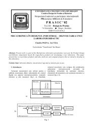
The third example is a four-bar mechanism, shown in Figure 4. The angular velocity ω of the left
crank is kinematically guided at a constant rate of 1 rad/s. Gravity effects are neglected. Bar lengths
are: AB=0.12 m; BC=0.24 m; CD=0.12 m; AD=0.24 m.
B
C
ω
5 o
A
D
Figure 4. Four-bar mechanism with assembly defect.
Typically, the axes of rotation of the four revolute joints are orthogonal to the plane of the
mechanism, and then it moves as a planar mechanism. However, in this case, the axis of rotation of
joint C is at a 5 degree angle with respect to the plane normal to simulate an assembly defect in the
mechanism. If the bars were rigid, no motion would be possible as the mechanism would lock. For
elastic bars, motion becomes possible, but generates large internal forces. Physical properties of the