real-time mbs formulations: towards virtual engineering

REAL-TIME MBS FORMULATIONS: TOWARDS VIRTUAL
ENGINEERING
J. Cuadrado, M. Gonzalez, R. Gutierrez, M.A. Naya
Laboratory of Mechanical Engineering, University of La Coruña, Ferrol, Spain
Abstract:
This paper presents the research conducted during the last years by the Laboratory of Mechanical Engineering
on real-time formulations for the dynamics of multi-body systems, a topic of great relevance for the
development of new virtual reality applications. The work carried out by our group has been focused on: a)
the development of real-time formulations capable of performing very fast calculations of the dynamics of
complex rigid-flexible multi-body systems; b) the experimental validation of the motions, deformations and
forces obtained through the application of the abovementioned formulations, so as to verify that reality is
being reasonably well imitated; c) the study of the aptitude of such formulations for becoming part of a virtual
reality environment, in connection with user-interface devices. In the paper, a real-time formulation developed
by the authors is described, along with some examples of rigid-flexible multi-body systems simulated with
such formulation. Moreover, results of the experimental validation of one of the examples are shown. Finally,
a simulator based on the proposed formulation is presented.
Key words: multi-body dynamics, real-time formulations, virtual reality, product life-cycle, experimental validation,
simulator.
1. INTRODUCTION
Entities in the real world can be considered from two points of view: graphical and physical. If a
virtual environment is to be created in which just the graphical aspect of objects is accounted for, only
the computer graphics discipline is needed. In such a virtual world, the user will be able to see, and
perhaps to hear, but never to touch or to be touched. Although these capabilities can be enough for
some applications, it is clear that they are far from replicating reality. On the other hand, a virtual
environment can be conceived in which objects possess physical properties, besides the graphical
ones, of course. Then, solids will experiment motion and/or deformation when forces act upon them,
and the user will be allowed to interact with its environment and to feel through the sense of touch too.
This virtual world is much closer to reality than the previously described one.
In order to develop environments with such types of capabilities, computational methods for the
dynamics of rigid-flexible multi-body systems will be demanded which encompass the two following
characteristics: a) adequate consideration of mechanical phenomena, like flexibility, contact, impact,
friction, damping, etc.; b) very fast calculation of all the kinematic and dynamic magnitudes
concerning the virtual bodies in the simulation and the user itself. Applications for physics-based
virtual environments can be very diverse, but undoubtedly some of them are fully related to the
product life-cycle: design (CAD), analysis (CAE), testing (CAT), manufacturing (CAM and CAPP),
maintenance and end-of-the-product. More specifically, the practical implementation of some ecodesign
concepts, like modularity, disassembling, reusability, recycling, new materials, low energy
consumption, noise reduction, low cost, integration of intelligent systems, security, etc., can benefit
from such applications.
Having the mentioned objectives in mind, the work carried out by our group has been focused on:
a) the development of real-time formulations capable of performing very fast calculations of the

170 J. Cuadrado, M. Gonzalez, R. Gutierrez, M.A. Naya
dynamics of complex rigid-flexible multi-body systems; b) the experimental validation of the motions,
deformations and forces obtained through the application of the abovementioned formulations, so as to
verify that reality is being reasonably well imitated; c) the study of the aptitude of such formulations
for becoming part of a virtual reality environment, in connection with user-interface devices.
The paper has been organized as follows: Section 2 describes a real-time formulation developed by
the authors for the dynamics of rigid-flexible multi-body systems; Section 3 shows some examples of
rigid-flexible multi-body systems simulated with such formulation, paying attention to the achieved
efficiency, robustness and accuracy; Section 4 reports the results of the experimental validation of one
of the examples; Section 5 presents a simulator based on the proposed formulation; and, finally,
Section 6 summarizes the conclusions of the work.
2. THE REAL-TIME FORMULATION
The three main elements (modeling, dynamic equations and numerical integrator) of the proposed
approach to solve the dynamics of rigid-flexible multi-body systems are described in what follows.
For the modeling, fully-Cartesian coordinates, also known as natural coordinates, are used. Both rigid
and flexible links are modeled with this type of coordinates in a total compatible form. Further
explanation about these coordinates can be found in [1]. The dynamic equations are stated through an
improved version of the index-3 augmented Lagrangian formulation with mass-orthogonal projections
given in [2]. For the integration scheme, the unconditionally-stable implicit single-step trapezoidal rule
has been chosen [3].
2.1 Modeling
The modeling of rigid bodies follows the general rules given in [1], and won’t be described here,
since it can be considered as a well established technique.
The modeling of flexible bodies is carried out by a floating frame of reference approach with
component mode synthesis for small elastic displacements. The global motion of each flexible body is
described as a superposition of the large-amplitude motion of a moving frame, rigidly attached to a
certain point of the body, and the small elastic displacements of the body with respect to an
undeformed configuration, taken as reference. Any deformed configuration of the body is expressed as
a linear combination of static and dynamic modes, in the sense of the mode synthesis approach with
fixed boundaries. The static modes depend on the natural coordinates defined at the joints of the body,
while the number of internal, dynamic modes should be decided by the analyst. A detailed description
of the kinematics of this method can be found in [4].
However, the approach proposed in the abovementioned reference for the dynamics has not been
adopted, as long as it showed to be too involved, particularly in what refers to the form of the inertia
terms. Therefore, the co-rotational approximation suggested in [5] has been considered in the way
proposed by [6] when natural coordinates are used for the modeling. This modified approach provides
the same level of accuracy while notably simplifying the formulation of the mass matrix and velocity
dependent forces vector. In what follows, the approach is
briefly described.
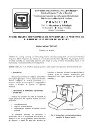
Figure 1 shows a general flexible body. Point r o
and
orthogonal unit vectors a, b and c serve to define the body
local reference frame, and are always needed, so that they
must compulsorily be considered as problem variables.
Additional points and unit vectors (further problem
variables) may be defined at the joints of the body (they
will produce the static modes) in the typical way featured
by the natural coordinates. The position of any point of the
Figure 1. General flexible body.
body can then be expressed as

Real-time MBS formulations: towards virtual engineering 171
r= r + A( r + u ), (1)
o
u
where r
o
is the position of the origin of the local reference frame, A the rotation matrix which
columns are the three orthogonal unit vectors a, b and c already mentioned, r u
the position of the
point in local coordinates for the undeformed configuration of the body, and u the elastic
displacement suffered by the point, also expressed in local coordinates. If the finite element method is
used, the elastic displacement can be written as
*
u = Nu , (2)
where N stands for the interpolation matrix which contains the interpolation functions, and
elastic displacements of the nodes. Substituting Eq. (2) into Eq. (1) yields
*
u are the
*
r = r + A(
r + Nu
) . (3)
o
u
At this point, the approach called co-rotational [5] is introduced. It implies the following
interpolation for the velocity of any point of the flexible body
*
r & = Nv , (4)
*
where v are the velocities of the nodes. Obviously, expression given by Eq. (4) for the velocities is
not consistent with expression given by Eq. (3) for the positions, as long as the former should be the
derivative of the latter.
Based on Eq. (4), the kinetic energy of the flexible body can be written in the form
1 1
T =
2
∫
&dm ∫
1
T
* T T *
* T
*
r & r = v N Nv dm = v M
FEMv
, (5)
2
2
v
v
where M
FEM
is the mass matrix of the finite element method. In order to express the kinetic energy in
terms of the problem variables, velocities of the nodes, v * , should be related with the problem
variables. Differentiating Eq. (3) and evaluating the result at the nodes gives
v
*
& & +
&
* *
= ro
+ A( ru
+ u ) Au
(6)
and considering that unit vectors a, b and c are the columns of rotation matrix A,
⎧ r&
o ⎫
⎪ ⎪
⎪
a&
⎪
⎧ v ⎫ ⎡I
a I a I a I A
0 ⎤⎪
b&
⎪
1
11 12 13
L L L
⎪ ⎪ ⎢
⎥⎪
⎪
⎢
⎥⎪
⎪
⎪
M
⎪
M
M
M c&
*
⎢
⎥
v = ⎨ ⎬ =
⎨u
&
, (7)
M M
M
M
1 ⎬
⎪ ⎪ ⎢
⎥
M
⎪ ⎪
⎪ ⎪ ⎢M
M
M ⎥ M
⎪ ⎪
⎪ ⎪ ⎢
⎥
⎩v
p ⎭ ⎣I
a
p1I
a
p2I
a
p3I
0 L L L A⎦⎪
M ⎪
⎪
M
⎪
⎪ ⎪
⎪
⎩u
&
p
⎪
⎭
where p is the number of nodes of the body, I the 3 by 3 identity matrix, and

172 J. Cuadrado, M. Gonzalez, R. Gutierrez, M.A. Naya
a
11
= r ux 1
+ u
x1
; a
12
= r uy 1
+ u
y1
; a
13
= r uz 1
+ u
z1
,
a = r + u
a = r + u
p1 uxp xp
;
p2 uyp yp
;
p uzp zp
a
3
= r + u . (8)
The elastic displacements can be expressed as superposition of static and dynamic modes,
ns
∑
i=
1
i
i
nd
∑
*
u = Ω η + Ψ ξ , (9)
j=
1
j
j
where n s and n d are the number of static and dynamic modes respectively, Ω
i
are the static modes, η i
are their amplitudes, Ψ
j
are the dynamic modes, and ξ j
are their amplitudes. Either the amplitudes of
the static modes as well as those of the dynamic modes are considered as problem variables.
Therefore, the problem variables for a general flexible body when using the proposed modeling
technique are: the origin of the local reference frame, r
o
, the thee orthogonal unit vectors, a, b, and c,
which define de local axes, and the amplitudes of static and dynamic modes, η i
and ξ j
, respectively.
Substituting Eq. (9) into Eq. (7) leads to
v
*
⎡I
⎢
⎢M
= ⎢M
⎢
⎢M
⎢
⎣
I
b
b
11
I
p1
I
b
b
12
I
p2
I
b
b
13
I
p3
I
AΩ
M
M
M
AΩ
1
1
p
1
...
...
AΩ
M
M
M
AΩ
1
ns
p
ns
AΨ
AΨ
1
1
p
1
...
...
AΨ
M
M
M
AΨ
1
nd
p
nd
⎧ r&
0 ⎫
⎪
a&
⎪
⎪ ⎪
⎪ b&
⎪
⎤⎪
⎪
⎥⎪
c&
⎪
⎥
⎪ & η
⎪
1
⎥⎨
⎬ = Bq&
, (10)
⎥⎪
M
⎪
⎥⎪
& η ⎪
⎥
ns
⎦⎪
& ⎪
⎪ ξ1
⎪
⎪ M ⎪
⎪
&
⎪
⎪⎩
ξn
⎪
d ⎭
r
where Ω
i
is a 3 by 1 vector containing static mode i evaluated at node r,
containing dynamic mode j evaluated at node s, and
s
Ψ
j
is a 3 by 1 vector
b
ns
nd
ns
nd
11
= rux
1
+ ∑ Ωix
1η
i
+ ∑Ψ
jx1ξ
j
; bp
1
= ruxp
+ ∑ Ωixpηi
+ ∑Ψ
jxpξ
j
,
i=
1
j=
1
i=
1
j=
1
b
ns
nd
ns
nd
12
= ruy1
+ ∑ Ωiy1η
i
+ ∑Ψ
jy1ξ
j
; bp2 = ruyp
+ ∑ Ωiypηi
+ ∑Ψ
jypξ
j
,
i=
1
j=
1
i=
1
j=
1
b
= r
+
ns
∑
Ω
η +
nd
∑
Ψ
ξ
13 uz1
iz1
i
jz1
j
;
p uzp
izp i
jzp j
i=
1
j=
1
i=
1
j=
1
ns
∑
nd
∑
b
3
= r + Ω η + Ψ ξ . (11)
The vector appearing in the right-hand-side of Eq. (10), q& , is the vector of the derivatives
*
(velocities) of the body variables q, and then, substituting the value of v given by this equation into
Eq. (5), the kinetic energy of the body can be written as

Real-time MBS formulations: towards virtual engineering 173
1 T T 1 T
T = q & B M Bq&
q&
Mq&
FEM
= , (12)
2
2
which means that the mass matrix of the general flexible body is given by the expression
T
M = B M B . (13)
FEM
Application of Lagrange equations with the kinetic energy of the flexible body given by Eq. (12)
leads to calculate the vector of velocity dependent inertia forces
Q v
T
= −B
M Bq & & . (14)
FEM
Therefore, it can be seen that, unlike their predecessors in [4], the final expressions for the inertia
terms obtained through the abovementioned approach, given by Eqs. (13) and (14), are compact and
relatively easy to evaluate.
2.2 Dynamic equations and numerical integrator
Once the modeling of a general flexible body has been explained, the approach to formulate the
dynamic equations of the whole multi-body system as well as the numerical procedure to integrate
them along the time is now addressed. Note that, as previously mentioned, either rigid and flexible
links can be combined in a totally compatible form when using the proposed formulation, so that the
actual mechanism can present both types of bodies.
The equations of motion of the whole multi-body system are given by an index-3 augmented
Lagrangian formulation in the form
T *
Mq& + Φ T
αΦ
+ Φ λ Q , (15)
q q
=
where M is the mass matrix, q& & are the accelerations, Φ
q
the Jacobian matrix of the constraint
*
equations, α the penalty factor, Φ the constraints vector, λ the Lagrange multipliers and Q the vector
of applied and velocity dependent inertia forces. The main sources of the constraints, grouped into
vector Φ, are: the rigid body conditions among the variables of each rigid body; the rigid body
conditions among the variables of the local reference frame of each flexible body, and among such
variables and those defining static modes whose deformation is to be neglected; the relative motion
conditions imposed by each joint among the variables of the two neighbor bodies connected by such
joint. The Lagrange multipliers are obtained from the following iteration process (given by sub-index
i, while sub-index n stands for time-step),
λ α , i=0,1,2,..., (16)
* *
i+ 1
= λ
i
+ Φi+
1
*
*
where the value of λ
o
is taken equal to the λ obtained in the previous time-step.
As integration scheme, the implicit single-step trapezoidal rule has been adopted. The
corresponding difference equations in velocities and accelerations are:
2
q
n
q
n
qˆ
⎛ ⎞
& &
+ 1
=
+ 1
+
n
with q & ˆ 2
n
= −⎜
q
n
+ q&
n ⎟ , (17)
∆t
⎝ ∆t ⎠
4
q& n
q
n
q&
ˆ
⎛
⎞
+ 1
=
2 + 1
+
n
with q && ˆ 4 4
n
= −⎜
q
n
+ q&
n
+ q&
n ⎟ . (18)
2
∆t
⎝ ∆t ∆t ⎠

174 J. Cuadrado, M. Gonzalez, R. Gutierrez, M.A. Naya
Dynamic equilibrium can be established at time-step n+1 by introducing the difference equations
(17) and (18) into the equations of motion (15), leading to
4
∆t
( Φ + λ ) − Q + Mq&
ˆ 0
T
2 n+ 1
+ Φ
1 + 1 + 1 + 1
=
n+
n n n
n
Mq &
q
α . (19)
For numerical reasons, the scaling of Eq. (19) by a factor of ∆t 2 /4 seems to be convenient, thus
yielding
2
2
2
∆t T
∆t ∆t
Mq ( ) ˆ
n+ 1
+ Φq α Φ
1
+
1
−
1
+ = 0
n+
1 n+
λ
n+
Q
n+
Mq&
n
, (20)
4
4 4
or, symbolically f ( q n+1
) = 0 .
In order to obtain the solution of this nonlinear system, the widely used iterative Newton-Raphson
method may be applied
( q)
⎡∂f
⎢
⎣ ∂q
⎤
⎥ ∆q
⎦
i
i +1
= −
being the residual vector
[ f ( q)
] i
, (21)
2
∆t
T
T *
[ f ( q)
] = ( Mq&&
+ Φ αΦ
+ Φ λ − Q)
4
q
q
(22)
and the approximated tangent matrix
⎡∂f
⎢
⎣ ∂q
2
( q) ⎤ ∆t ∆t T
= M + C + ( Φ αΦ
K)
⎥
⎦
2
4
q q
+
, (23)
where C and K represent the contribution of damping and elastic forces of the system provided they
exist.
A closer look at the tangent matrix reveals that ill-conditioning may appear when the time-step
becomes small. It may be seen in Eq. (23) that K and the constraint terms are multiplied by ∆t 2 , C by
∆t and M is not affected by the step size. As a consequence when ∆t reaches small values, large roundoff
errors will occur. In fact, it has been demonstrated in [7] that for an index-3 differential-algebraic
equation, the tangent matrix has a condition number of order 1/∆t 3 . Consequently, the method is
bound to have round-off errors for step sizes smaller than 10 -5 , which lets a sufficient range for
solving practical problems.
The procedure explained above yields a set of positions q
n+ 1 that not only satisfies the equations
of motion (19), but also the constraint condition Φ = 0 . However, it is not expected that the
corresponding sets of velocities and accelerations satisfy Φ & = 0 and Φ &
= 0 , because these conditions
have not been imposed in the solution process. To overcome this difficulty, mass-damping-stiffnessorthogonal
projections in velocities and accelerations are performed. It can be seen that the projections
leading matrix is the same tangent matrix appearing in Eq. (23). Therefore, triangularization is avoided
and projections in velocities and accelerations are carried out with just forward reductions and back
substitutions.
*
If q& and q& & * are the velocities and accelerations obtained after convergence has been achieved in
the Newton-Raphson iteration, their cleaned counterparts q& and q& & are calculated from

Real-time MBS formulations: towards virtual engineering 175
2
2
2
∆t
∆t
T
∆t
∆t
* ∆t
T
[ M + C + ( Φ
qαΦ
q
+ K)]
q& = [ M + C + K]
q&
− Φ
qαΦ
t
, (24)
2 4
2 4 4
for the velocities, and
2
2
2
∆t
∆t
T
∆t
∆t
* ∆t
T
[ M + C + ( Φ
qα Φ
q
+ K)]
q&
= [ M + C + K]
q&&
− Φ
qα(
Φ&
qq&
+ Φ&
t
) , (25)
2 4
2 4 4
for the accelerations.
Sparse matrix technology can be implemented to solve all the linear sets of equations that arise
when applying this method, provided the size of the system is large enough for such technique to be
worthwhile. The fact that the leading matrix is symmetric and positive-definite can be taken into
T
T
account as well. The products B M
FEMB
and B M B&
q&
FEM
for each flexible body and ΦqΦ
T
q
for
the whole system, can also be optimized by considering the sparse character of the matrices.
3. EXAMPLES
In order to show the behavior of the described formulation, the following examples of rigid and
flexible multi-body systems have been solved. In all cases, the simulations have been run on common
personal computers. Based on the obtained results, the performance of the method is evaluated in
terms of efficiency, robustness and accuracy.
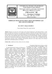
3.1 Double four-bar planar mechanism
The first example is a one degree-of-freedom assembly
of two four-bar linkages, illustrated in Figure 2, which has
been proposed [8] as an example to test the performance in
cases where the mechanism undergoes singular
configurations. When the mechanism reaches a horizontal
position, the number of degrees of freedom instantaneously
increases from 1 to 3. All the links have a uniformly
distributed unit mass and a unit length. The gravity force Figure 2. Double four-bar mechanism
acts in the negative vertical direction. At the beginning, the
links pinned to the ground are in vertical position and upwards, receiving a unit clockwise angular
velocity. The simulation lasts for 10 s, during which the mechanism goes through the singular position
ten times..
Table 1 shows the obtained results for different time-steps (∆t). The error is measured as the
maximum deviation, in J, suffered by the system energy.
Table 1. Error and CPU-time for the double four-bar mechanism.
∆t (s) Error (J) CPU-time (s)
0.01 -0.21 0.86
0.03 -0.83 0.37
0.05 -9.03 0.26
0.1 wrong results wrong results
As it can be seen in Table 1, the formulation shows a robust behavior when facing singular
configurations, and large time-steps can be taken with acceptable accuracy. Regarding the efficiency,
the example has been implemented in the computing environment Matlab. Although real-time
performance is achieved, the reported CPU-times would be drastically reduced if the same programs
were written in Fortran or C languages.

176 J. Cuadrado, M. Gonzalez, R. Gutierrez, M.A. Naya
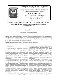
3.2 Serial robot
The PUMA robot, designed by Unimation & Co. and shown in Figure 3, is an example of a 6
degrees-of-freedom serial manipulator. It has been often used by different authors [9] to illustrate
methods and procedures in several areas of robotics. In this work, the robot has been taken as an
example of multibody system undergoing changing configurations.
Starting from rest, torques at the six hinges of the robot are provided so that, in a time of 2 s, it
arrives at a new position in the space, again in rest conditions. Once
the new position has been reached, a point of the hand is attached to
the ground, so that the robot loses 3 degrees-of-freedom. In this
new configuration, torques are applied to the three rotational pairs
of the hand, and a second maneuver, which lasts 4 s and ends with
rest conditions, is performed. Finally, the robot is released from its
attachment and returned in 2 s to the initial position by torques
acting at the six revolute joints, once more finishing the maneuver
at rest conditions. Therefore, the total simulation time is 8 s.
Table 2 illustrates the results obtained when applying the
proposed method. The error has been calculated as the distance, in
Figure 3. PUMA robot
mm, between the hand positions at initial and final times (which,
ideally, should be coincident).
Table 2. Error and CPU-time for the PUMA robot.
∆t (s) Error (mm) CPU-time (s)
0.01 0.53 6.25
0.05 3.4 1.92
0.1 no convergence no convergence
From the results reported in Table 2, it is obvious that the formulation deals well with changing
configurations. As in the previous example, large time-steps can be taken with acceptable accuracy.
Although the example has been implemented in the computing environment Matlab, real-time
performance is comfortably achieved.
3.3 Four-bar mechanism with assembly defect
The third example is a four-bar mechanism, shown in Figure 4. The angular velocity ω of the left
crank is kinematically guided at a constant rate of 1 rad/s. Gravity effects are neglected. Bar lengths
are: AB=0.12 m; BC=0.24 m; CD=0.12 m; AD=0.24 m.
B
C
ω
5 o
A
D
Figure 4. Four-bar mechanism with assembly defect.
Typically, the axes of rotation of the four revolute joints are orthogonal to the plane of the
mechanism, and then it moves as a planar mechanism. However, in this case, the axis of rotation of
joint C is at a 5 degree angle with respect to the plane normal to simulate an assembly defect in the
mechanism. If the bars were rigid, no motion would be possible as the mechanism would lock. For
elastic bars, motion becomes possible, but generates large internal forces. Physical properties of the

Real-time MBS formulations: towards virtual engineering 177
bars are: mass density 3000 Kg/m 3 , modulus of elasticity 7x10 10 N/m 2 , Poisson modulus 0.33. The
section of the bars is circular with a diameter of 5 mm. For this example, the objective is to simulate
10 seconds of motion.
6,00E+00
4,00E+00
2,00E+00
0,00E+00
-2,00E+00
-4,00E+00
FEA (T)
FEA (My)
FEA (Mz)
-6,00E+00
-8,00E+00
-1,00E+01
0,00 2,00 4,00 6,00 8,00 10,00
Time (s)
Figure 5. Torsion and bending moments at the middle section of the coupler: a) Proposed method; b) Finite element
commercial code.
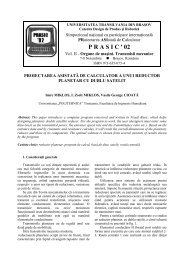
3.4 Prototype car
A prototype car, which can be seen in Figure 6, has
been manufactured in steel tubing and parts from old cars
have been cannibalized and conveniently adapted (i.e.
engine, suspension and steering systems, wheels, etc.).
The total mass of the car is 597 kg. Front shockabsorbers
are characterized by a stiffness constant of
12360 N/m and a free length of 0.750 m, while their rear
counterparts have values of 10595 N/m and 0.916 m for
the same magnitudes. Damping of these front and rear
elements has been set to 1000 Ns/m. Radii of the tires are
0.27 and 0.29 m for the front and rear tires respectively,
which show a vertical stiffness of 60000 N/m.
Figure 6. The prototype car.
The example has been used in two different ways
corresponding to different purposes.
On one hand, the computer model of the car has been generated, considering the chassis as a
flexible body, so that the stresses suffered by such body along the motion could be calculated, and
compared with their experimentally measured counterparts. Therefore, the first purpose was the
experimental validation of the proposed formulation.
On the other hand, a second computer model of the car has been implemented, but this time all the
system bodies have been taken as rigid. This model has served as the calculation engine of a driving
simulator, so as to verify whether the proposed formulation was reliable when integrated in an
interactive real-time application.
A detailed description of each study is given in the following Sections.
4. EXPERIMENTAL VALIDATION
A maneuver has been defined in order to compare the resulting stresses at the chassis coming from
measurement and simulation: starting from rest, the car accelerates and travels direct until reaching an
approximate speed of 5 m/s, then drops down a curb of 8 cm height, and finally brakes until complete

178 J. Cuadrado, M. Gonzalez, R. Gutierrez, M.A. Naya
stop is attained. In this way, the bending modes of the chassis are excited. The described maneuver is
illustrated in Figure 7.
To obtain the motion of the car, four tri-axial
accelerometers have been attached to the chassis at the four
corners of its base. Accelerations provided by the sensors
in the motion direction have been integrated twice in order
to obtain the position and velocity of the chassis at all
times. On the other hand, four Wheatstone bridges have
been installed at four points of the chassis to measure
bending stresses. They are half-bridges, with an upper and
a lower band each, to measure the normal bending stresses
on the steel tubes surfaces. The sixteen captured signals –
twelve accelerations and four strains– were recorded by a
laptop PC after passing through a data-adquisition board..
The actual maneuver of 15 s has been simulated by
implementation of the proposed formulation, with a fixed time-step of 0.01 s, the same sample period
used for data adquisition during the experimental test, where a low-pass filter was applied with a
cutoff frequency of 10 Hz to avoid noise from engine vibration.
4.1 Accuracy
Figure 7. The maneuver
The comparison between measured and calculated bending moments at a certain point of the
chassis is shown in Figure 8. At the view of the results, three time intervals can be distinguished.
The first one is the [0,5] interval. During this period of time, the car is at rest, but some peaks can
be detected at about 2 s. They are explained because, at that time, the gear was set on drive position.
This kind of engine loads is not considered by the model
since engine torque is derived from acceleration
information. Therefore, if the car is at rest, no engine
torque is introduced in the model. This fact justifies the
discrepancies shown between measurements and
calculations during this time interval.
The second time interval is [5, 10]. During this five
seconds, the car accelerates, goes over the curb, and
brakes until reaching the rest again. Good correlation is
found during the accelerating and braking phases. The
high peaks due to the falling action are not perfectly
reproduced, although their intensities are reasonably
Figure 8. Comparison of bending moments
captured. An explanation for such peak discrepancy can
be the appearance of percussional forces in the actual
prototype, due to the presence of clearances in some joints which have not been modeled.
The third and final time interval is [10, 15], when the vehicle is again at rest. Some amount of error
in the measurements can be detected in the figures, since the bending moments should return to zero,
given that the initial and final positions of the car are exactly the same. However, the calculations
come back correctly to zero.
4.2 Efficiency and robustness
The proposed formulation has shown an efficient behavior in the analysis of this case-study. The
method was implemented on Fortran language, and the CPU time spent to run this 15-secondsimulation
was 48 s, that is, only a factor of 3 to real-time performance. The average number of
Newton-Raphson iterations to attain convergence into each time-step of 0.01 s was equal to 2, needing
a maximum of 3 iterations at the more difficult points.

Real-time MBS formulations: towards virtual engineering 179
Some important figures should be taken into account to adequately appraise the performance of the
method. The number of problem variables is 293, related through 239 constraints, which means that 2
x 293 = 586 variables (positions and velocities) are integrated along the time, and that the Φ
q
matrix
size is (239 x 293), which in turn determines the cost of the product ΦqΦ
T
q
. The number of degrees of
freedom of the chassis finite element model is 1266, while the number of static plus dynamic modes is
65, so that the M
FEM
matrix size is (1266 x 1266) and the B matrix size is (1266 x 77). Therefore,
T
T
both products B M
FEMB
and B M B&
q&
FEM
are also rather time-consuming. Undoubtedly, as many
readers can think when considering the adopted modeling, an effort could be done in order to reduce
all these figures, since a special emphasis on keeping the problem size as small as possible has not
been carried out. Consequently, perhaps the efficiency could be slightly enhanced, but probably the
improvement would not be significant and, what is more important, it would not contribute to better
show the power of the method, which was the objective of this work.
On the other hand, and this also affects to robustness consideration, the performed maneuver is
particularly violent, since the curb descent produces high values of vertical acceleration. Moreover, the
kinematic guidance of the forward motion of the prototype shows a curly shape which supposes an
additional difficulty for the numerical integration.
5. DRIVING SIMULATOR
The computational model of the car has been used
to create a driving simulator, shown in Figure 9, by
combining the already mentioned vehicle dynamics
code, along with realistic graphical output and gametype
driving peripherals (steering wheel and pedals).
The proposed formulation has shown to be
efficient enough to enable the interactive driving of
the car, and robust enough to bear very long driving
sessions (over 1000 s), not free of violent maneuvers
like jumps from elevated positions to the ground or
sudden turns.
6. CONCLUSIONS
Figure 9. Driving simulator
Based on the results, the following conclusions may be established:
1. A real-time formulation has been developed capable of performing very fast calculations of the
dynamics of complex rigid-flexible multi-body systems.
2. The modeling is carried out with natural coordinates, making use of the floating frame of reference
approach with static and dynamic modes for the flexible bodies, along with the co-rotational
approach to simplify the inertial terms.
3. The equations of motion are stated through an index-3 augmented Lagrangian scheme, which is
combined with the implicit, single-step, trapezoidal rule to perform the numerical integration. Massdamping-stiffness-orthogonal
projections in velocities and accelerations are needed at each timestep
to provide stability.
4. The formulation is global and, therefore, very easy to implement. This fact represents an advantage
with respect to topological formulations, often used for real-time purposes.
5. The formulation provides good levels of efficiency, robustness and accuracy, as demonstrated
through the solved examples. It can handle singular positions, changing configurations, stiff systems
and large models.
6. The formulation has been experimentally validated through the comparison between calculated and
measured stresses on a component of a complex and realistic multi-body system.

180 J. Cuadrado, M. Gonzalez, R. Gutierrez, M.A. Naya
7. The formulation has shown to be valid for becoming part of a virtual reality environment, in
connection with user-interface devices, since it has successfully served as the calculation engine for
a driving simulator.
8. Therefore, it can be affirmed that the presented formulation is a good candidate for future virtual
engineering applications.
REFERENCES
1. GARCIA DE JALON, J., BAYO, E., “Kinematic and Dynamic Simulation of Multibody Systems –The Real-Time
Challenge”, Springer-Verlag, 1994.
2. BAYO, E., LEDESMA, R., “Augmented Lagrangian and Mass-Orthogonal Projection Methods for Constrained
Multibody Dynamics”, Nonlinear Dynamics, Vol. 9, 1996, pp. 113-130.
3. EICH-SOELLNER, E., FÜHRER, C., “Numerical Methods in Multibody Dynamics”, B.G. Teubner Stuttgart, 1998.
4. CUADRADO, J., CARDENAL, J., GARCIA DE JALON, J., “Flexible Mechanisms through Natural Coordinates and
Component Synthesis: An Approach Fully Compatible with the Rigid Case”, Int. Journal for Numerical Methods in
Engineering, Vol. 39, No. 20, 1996, pp. 3535-3551.
5. GERADIN, M., CARDONA, A., “Flexible Multibody Dynamics -A Finite Element Approach”, John Wiley and Sons,
2001.
6. AVELLO, A., “Simulación Dinámica Interactiva de Mecanismos Flexibles con Pequeñas Deformaciones”, Ph. D. Thesis,
Universidad de Navarra, Spain, 1995.
7. BRENAN, K.E., CAMPBELL, S.L., PETZOLD, L.R., “The Numerical Solution of Initial Value Problems in Differential-
Algebraic Equations”, Elsevier, 1989.
8. BAYO, E., AVELLO, A., “Singularity Free Augmented Lagrangian Algorithms for Constrained Multibody Dynamics”,
Nonlinear Dynamics, Vol. 5, 1994, pp. 209-231.
9. ANGELES, J., MA, O., “Dynamic Simulation of n-axis Serial Robotic Manipulators using a Natural Orthogonal
Complement”, Int. J. of Robotic Research, Vol. 7, No. 5, 1988, pp. 32-47.