Electromagnetic Fields and Energy - Chapter 5 ... - MIT

MIT OpenCourseWare 

http://ocw.mit.edu 

Haus, Hermann A., and James R. Melcher. Electromagnetic Fields and Energy. 

Englewood Cliffs, NJ: Prentice-Hall, 1989. ISBN: 9780132490207. 

Please use the following citation format: 

Haus, Hermann A., and James R. Melcher, Electromagnetic Fields and 

Energy. (Massachusetts Institute of Technology: MIT 

OpenCourseWare). http://ocw.mit.edu (accessed [Date]). License: 

Creative Commons Attribution-NonCommercial-Share Alike. 

Also available from Prentice-Hall: Englewood Cliffs, NJ, 1989. ISBN: 

9780132490207. 

Note: Please use the actual date you accessed this material in your citation. 

For more information about citing these materials or our Terms of Use, visit: 

http://ocw.mit.edu/terms

5 

ELECTROQUASISTATIC 

FIELDS FROM THE 

BOUNDARY VALUE 

POINT OF VIEW 

5.0 INTRODUCTION 

The electroquasistatic laws were discussed in Chap. 4. The electric field intensity 

E is irrotational and represented by the negative gradient of the electric potential. 

E = −Φ 

(1) 

Gauss’ law is then satisfied if the electric potential Φ is related to the charge density 

ρ by Poisson’s equation 

2 ρ 

Φ = − (2) 

 

In chargefree regions of space, Φ obeys Laplace’s equation, (2), with ρ = 0. 

The last part of Chap. 4 was devoted to an “opportunistic” approach to 

finding boundary value solutions. An exception was the numerical scheme described 

in Sec. 4.8 that led to the solution of a boundary value problem using the sourcesuperposition 

approach. In this chapter, a more direct attack is made on solving 

boundary value problems without necessarily resorting to numerical methods. It is 

one that will be used extensively not only as effects of polarization and conduction 

are added to the EQS laws, but in dealing with MQS systems as well. 

Once again, there is an analogy useful for those familiar with the description 

of linear circuit dynamics in terms of ordinary differential equations. With time as 

the independent variable, the response to a drive that is turned on when t = 0 can 

be determined in two ways. The first represents the response as a superposition of 

impulse responses. The resulting convolution integral represents the response for 

all time, before and after t = 0 and even when t = 0. This is the analogue of the 

point of view taken in the first part of Chap. 4. 

The second approach represents the history of the dynamics prior to when 

t = 0 in terms of initial conditions. With the understanding that interest is confined 

to times subsequent to t = 0, the response is then divided into “particular” 

1 

o

2 Electroquasistatic Fields from the Boundary Value Point of View Chapter 5 

and “homogeneous” parts. The particular solution to the differential equation representing 

the circuit is not unique, but insures that at each instant in the temporal 

range of interest, the differential equation is satisfied. This particular solution need 

not satisfy the initial conditions. In this chapter, the “drive” is the charge density, 

and the particular potential response guarantees that Poisson’s equation, (2), is 

satisfied everywhere in the spatial region of interest. 

In the circuit analogue, the homogeneous solution is used to satisfy the initial 

conditions. In the field problem, the homogeneous solution is used to satisfy 

boundary conditions. In a circuit, the homogeneous solution can be thought of as 

the response to drives that occurred prior to when t = 0 (outside the temporal 

range of interest). In the determination of the potential distribution, the homogeneous 

response is one predicted by Laplace’s equation, (2), with ρ = 0, and can be 

regarded either as caused by fictitious charges residing outside the region of interest 

or as caused by the surface charges induced on the boundaries. 

The development of these ideas in Secs. 5.1–5.3 is selfcontained and does not 

depend on a familiarity with circuit theory. However, for those familiar with the 

solution of ordinary differential equations, it is satisfying to see that the approaches 

used here for dealing with partial differential equations are a natural extension of 

those used for ordinary differential equations. 

Although it can often be found more simply by other methods, a particular 

solution always follows from the superposition integral. The main thrust of 

this chapter is therefore toward a determination of homogeneous solutions, of finding 

solutions to Laplace’s equation. Many practical configurations have boundaries 

that are described by setting one of the coordinate variables in a threedimensional 

coordinate system equal to a constant. For example, a box having rectangular crosssections 

has walls described by setting one Cartesian coordinate equal to a constant 

to describe the boundary. Similarly, the boundaries of a circular cylinder are naturally 

described in cylindrical coordinates. So it is that there is great interest in having 

solutions to Laplace’s equation that naturally “fit” these configurations. With 

many examples interwoven into the discussion, much of this chapter is devoted to 

cataloging these solutions. The results are used in this chapter for describing EQS 

fields in free space. However, as effects of polarization and conduction are added 

to the EQS purview, and as MQS systems with magnetization and conduction are 

considered, the homogeneous solutions to Laplace’s equation established in this 

chapter will be a continual resource. 

A review of Chap. 4 will identify many solutions to Laplace’s equation. As 

long as the field source is outside the region of interest, the resulting potential obeys 

Laplace’s equation. What is different about the solutions established in this chapter? 

A hint comes from the numerical procedure used in Sec. 4.8 to satisfy arbitrary 

boundary conditions. There, a superposition of N solutions to Laplace’s equation 

was used to satisfy conditions at N points on the boundaries. Unfortunately, to 

determine the amplitudes of these N solutions, N equations had to be solved for 

N unknowns. 

The solutions to Laplace’s equation found in this chapter can also be used as 

the terms in an infinite series that is made to satisfy arbitrary boundary conditions. 

But what is different about the terms in this series is their orthogonality. This 

property of the solutions makes it possible to explicitly determine the individual 

amplitudes in the series. The notion of the orthogonality of functions may already

Sec. 5.1 

Particular and Homogeneous Solutions 

3 

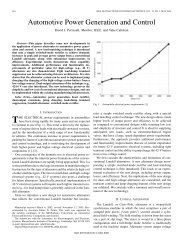
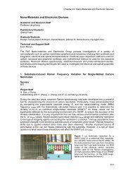
Fig. 5.1.1 Volume of interest in which there can be a distribution of charge 

density. To illustrate bounding surfaces on which potential is constrained, n 

isolated surfaces and one enclosing surface are shown. 

be familiar through an exposure to Fourier analysis. In any case, the fundamental 

ideas involved are introduced in Sec. 5.5. 

5.1 PARTICULAR AND HOMOGENEOUS SOLUTIONS TO POISSON’S 

AND LAPLACE’S EQUATIONS 

Suppose we want to analyze an electroquasistatic situation as shown in Fig. 5.1.1. 

A charge distribution ρ(r) is specified in the part of space of interest, designated 

by the volume V . This region is bounded by perfect conductors of specified shape 

and location. Known potentials are applied to these conductors and the enclosing 

surface, which may be at infinity. 

In the space between the conductors, the potential function obeys Poisson’s 

equation, (5.0.2). A particular solution of this equation within the prescribed volume 

V is given by the superposition integral, (4.5.3). 

 

ρ(r )dv 

Φ p (r) = (1) 

V 4π o|r − r | 

 

This potential obeys Poisson’s equation at each point within the volume V . Since we 

do not evaluate this equation outside the volume V , the integration over the sources 

called for in (1) need include no sources other than those within the volume V . This 

makes it clear that the particular solution is not unique, because the addition to 

the potential made by integrating over arbitrary charges outside the volume V will 

only give rise to a potential, the Laplacian derivative of which is zero within the 

volume V . 

Is (1) the complete solution? Because it is not unique, the answer must be, 

surely not. Further, it is clear that no information as to the position and shape of 

the conductors is built into this solution. Hence, the electric field obtained as the 

negative gradient of the potential Φ p of (1) will, in general, possess a finite tangential 

component on the surfaces of the electrodes. On the other hand, the conductors


have surface charge distributions which adjust themselves so as to cause the net 

electric field on the surfaces of the conductors to have vanishing tangential electric 

field components. The distribution of these surface charges is not known at the 

outset and hence cannot be included in the integral (1). 

A way out of this dilemma is as follows: The potential distribution we seek 

within the space not occupied by the conductors is the result of two charge distributions. 

First is the prescribed volume charge distribution leading to the potential 

function Φ p , and second is the charge distributed on the conductor surfaces. The potential 

function produced by the surface charges must obey the sourcefree Poisson’s 

equation in the space V of interest. Let us denote this solution to the homogeneous 

form of Poisson’s equation by the potential function Φ h . Then, in the volume V, Φ h 

must satisfy Laplace’s equation. 

2 Φ h = 0 (2) 

The superposition principle then makes it possible to write the total potential as 

Φ = Φ p + Φ h (3) 

The problem of finding the complete field distribution now reduces to that of 

finding a solution such that the net potential Φ of (3) has the prescribed potentials 

v i on the surfaces S i . Now Φ p is known and can be evaluated on the surface S i . 

Evaluation of (3) on S i gives 

v i = Φ p (S i ) + Φ h (S i ) (4) 

so that the homogeneous solution is prescribed on the boundaries S i . 

Φ h (S i ) = v i − Φ p (S i ) (5) 

Hence, the determination of an electroquasistatic field with prescribed potentials 

on the boundaries is reduced to finding the solution to Laplace’s equation, (2), that 

satisfies the boundary condition given by (5). 

The approach which has been formalized in this section is another point of 

view applicable to the boundary value problems in the last part of Chap. 4. Certainly, 

the abstract view of the boundary value situation provided by Fig. 5.1.1 is 

not different from that of Fig. 4.6.1. In Example 4.6.4, the field shown in Fig. 4.6.8 

is determined for a point charge adjacent to an equipotential chargeneutral spherical 

electrode. In the volume V of interest outside the electrode, the volume charge 

distribution is singular, the point charge q. The potential given by (4.6.35), in fact, 

takes the form of (3). The particular solution can be taken as the first term, the 

potential of a point charge. The second and third terms, which are equivalent to 

the potentials caused by the fictitious charges within the sphere, can be taken as 

the homogeneous solution. 

Superposition to Satisfy Boundary Conditions. In the following sections, 

superposition will often be used in another way to satisfy boundary conditions.

Sec. 5.2 

Uniqueness of Solutions 

5 

Suppose that there is no charge density in the volume V , and again the potentials 

on each of the n surfaces S j are v j . Then 

2 Φ = 0 (6) 

Φ = v j on S j , j = 1, . . . n (7) 

The solution is broken into a superposition of solutions Φ j that meet the required 

condition on the jth surface but are zero on all of the others. 

n 

Φ = 

 

Φj (8) 

j=1 

Φ j ≡ 

 

vj 

on S j 

0 on S 1 . . . S j−1 , S j+1 . . . S 

(9) 

n 

Each term is a solution to Laplace’s equation, (6), so the sum is as well. 

2 Φ j = 0 (10) 

In Sec. 5.5, a method is developed for satisfying arbitrary boundary conditions on 

one of four surfaces enclosing a volume of interest. 

Capacitance Matrix. Suppose that in the n electrode system the net charge 

on the ith electrode is to be found. In view of (8), the integral of E · da over the 

surface S i enclosing this electrode then gives 

 

 

 

n 

q i = − o Φ · da = − o Φj · da (11) 

S i S i j=1 

Because of the linearity of Laplace’s equation, the potential Φ j is proportional to 

the voltage exciting that potential, v j . It follows that (11) can be written in terms 

of capacitance parameters that are independent of the excitations. That is, (11) 

becomes 

n 

q i = 

 

Cij v j (12) 

where the capacitance coefficients are 

j=1 

− da 

S 

C ij = i 

o Φ j · 

v j 

(13) 

The charge on the ith electrode is a linear superposition of the contributions of 

all n voltages. The coefficient multiplying its own voltage, C ii , is called the selfcapacitance, 

while the others, C ij , i = j, are the mutual capacitances.


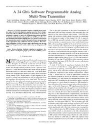
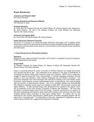
Fig. 5.2.1 Field line originating on one part of bounding surface and terminating 

on another after passing through the point r o . 

5.2 UNIQUENESS OF SOLUTIONS TO POISSON’S EQUATION 

We shall show in this section that a potential distribution obeying Poisson’s equation 

is completely specified within a volume V if the potential is specified over the 

surfaces bounding that volume. Such a uniqueness theorem is useful for two reasons: 

(a) It tells us that if we have found such a solution to Poisson’s equation, whether 

by mathematical analysis or physical insight, then we have found the only solution; 

and (b) it tells us what boundary conditions are appropriate to uniquely specify a 

solution. If there is no charge present in the volume of interest, then the theorem 

states the uniqueness of solutions to Laplace’s equation. 

Following the method “reductio ad absurdum”, we assume that the solution 

is not unique– that two solutions, Φ a and Φ b , exist, satisfying the same boundary 

conditions– and then show that this is impossible. The presumably different solutions 

Φ a and Φ b must satisfy Poisson’s equation with the same charge distribution 

and must satisfy the same boundary conditions. 

2 ρ 

Φ a = − ; Φ a = Φ i on S i (1) 

 

o 

2 ρ 

Φ b = − ; Φ b = Φ i on S i (2) 

 

o 

It follows that with Φ d defined as the difference in the two potentials, Φ d = Φ a −Φ b , 

2 Φ d ≡ · (Φ d ) = 0; Φ d = 0 on S i (3) 

A simple argument now shows that the only way Φ d can both satisfy Laplace’s 

equation and be zero on all of the bounding surfaces is for it to be zero. First, it 

is argued that Φ d cannot possess a maximum or minimum at any point within V . 

With the help of Fig. 5.2.1, visualize the negative of the gradient of Φ d , a field line, 

as it passes through some point r o . Because the field is solenoidal (divergence free), 

such a field line cannot start or stop within V (Sec. 2.7). Further, the field defines a 

potential (4.1.4). Hence, as one proceeds along the field line in the direction of the 

negative gradient, the potential has to decrease until the field line reaches one of 

the surfaces S i bounding V . Similarly, in the opposite direction, the potential has 

to increase until another one of the surfaces is reached. Accordingly, all maximum 

and minimum values of Φ d (r) have to be located on the surfaces.

Sec. 5.3 

Continuity Conditions 

7 

The difference potential at any interior point cannot assume a value larger 

than or smaller than the largest or smallest value of the potential on the surfaces. 

But the surfaces are themselves at zero potential. It follows that the difference 

potential is zero everywhere in V and that Φ a = Φ b . Therefore, only one solution 

exists to the boundary value problem stated with (1). 

5.3 CONTINUITY CONDITIONS 

At the surfaces of metal conductors, charge densities accumulate that are only a 

few atomic distances thick. In describing their fields, the details of the distribution 

within this thin layer are often not of interest. Thus, the charge is represented by 

a surface charge density (1.3.11) and the surface supporting the charge treated as 

a surface of discontinuity. 

In such cases, it is often convenient to divide a volume in which the field 

is to be determined into regions separated by the surfaces of discontinuity, and to 

use piecewise continuous functions to represent the fields. Continuity conditions are 

then needed to connect field solutions in two regions separated by the discontinuity. 

These conditions are implied by the differential equations that apply throughout 

the region. They assure that the fields are consistent with the basic laws, even in 

passing through the discontinuity. 

Each of the four Maxwell’s equations implies a continuity condition. Because 

of the singular nature of the source distribution, these laws are used in integral form 

to relate the fields to either side of the surface of discontinuity. With the vector n 

defined as the unit normal to the surface of discontinuity and pointing from region 

(b) to region (a), the continuity conditions were summarized in Table 1.8.3. 

In the EQS approximation, the laws of primary interest are Faraday’s law 

without the magnetic induction and Gauss’ law, the first two equations of Chap. 4. 

Thus, the corresponding EQS continuity conditions are 

n × [E a − E b ] = 0 (1) 

n · ( o E a − o E b ) = σ s (2) 

Because the magnetic induction makes no contribution to Faraday’s continuity condition 

in any case, these conditions are the same as for the general electrodynamic 

laws. As a reminder, the contour enclosing the integration surface over which Faraday’s 

law was integrated (Sec. 1.6) to obtain (1) is shown in Fig. 5.3.1a. The integration 

volume used to obtain (2) from Gauss’ law (Sec. 1.3) is similarly shown in 

Fig. 5.3.1b. 

What are the continuity conditions on the electric potential? The potential Φ 

is continuous across a surface of discontinuity even if that surface carries a surface 

charge density. This will be the case when the E field is finite (a dipole layer 

containing an infinite field causes a jump of potential), because then the line integral 

of the electric field from one side of the surface to the other side is zero, the pathlength 

being infinitely small. 

Φ a − Φ b = 0 (3) 

To determine the jump condition representing Gauss’ law through the surface 

of discontinuity, it was integrated (Sec. 1.3) over the volume shown intersecting the


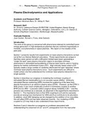
Fig. 5.3.1 (a) Differential contour intersecting surface supporting surface 

charge density. (b) Differential volume enclosing surface charge on surface having 

normal n. 

surface in Fig. 5.3.1b. The resulting continuity condition, (2), is written in terms 

of the potential by recognizing that in the EQS approximation, E = −Φ. 

n · [(Φ) a − (Φ) b ] = − σ o 

s 

(4) 

At a surface of discontinuity that carries a surface charge density, the normal 

derivative of the potential is discontinuous. 

The continuity conditions become boundary conditions if they are made to 

represent physical constraints that go beyond those already implied by the laws 

that prevail in the volume. A familiar example is one where the surface is that of 

an electrode constrained in its potential. Then the continuity condition (3) requires 

that the potential in the volume adjacent to the electrode be the given potential 

of the electrode. This statement cannot be justified without invoking information 

about the physical nature of the electrode (that it is “infinitely conducting,” for 

example) that is not represented in the volume laws and hence is not intrinsic to 

the continuity conditions. 

5.4 SOLUTIONS TO LAPLACE’S EQUATION IN CARTESIAN 

COORDINATES 

Having investigated some general properties of solutions to Poisson’s equation, it is 

now appropriate to study specific methods of solution to Laplace’s equation subject 

to boundary conditions. Exemplified by this and the next section are three standard 

steps often used in representing EQS fields. First, Laplace’s equation is set up in the 

coordinate system in which the boundary surfaces are coordinate surfaces. Then, 

the partial differential equation is reduced to a set of ordinary differential equations 

by separation of variables. In this way, an infinite set of solutions is generated. 

Finally, the boundary conditions are satisfied by superimposing the solutions found 

by separation of variables. 

In this section, solutions are derived that are natural if boundary conditions 

are stated along coordinate surfaces of a Cartesian coordinate system. It is assumed 

that the fields depend on only two coordinates, x and y, so that Laplace’s equation

Sec. 5.4 

Solutions to Laplace’s Equation 

9 

is (Table I) 

∂ 2 Φ ∂ 2 Φ 

+ = 0 (1) 

∂x 2 ∂y 2 

This is a partial differential equation in two independent variables. One timehonored 

method of mathematics is to reduce a new problem to a problem previously 

solved. Here the process of finding solutions to the partial differential equation is 

reduced to one of finding solutions to ordinary differential equations. This is accomplished 

by the method of separation of variables. It consists of assuming solutions 

with the special space dependence 

Φ(x, y) = X(x)Y (y) (2) 

In (2), X is assumed to be a function of x alone and Y is a function of y alone. 

If need be, a general space dependence is then recovered by superposition of these 

special solutions. Substitution of (2) into (1) and division by Φ then gives 

1 d 2 X(x) 1 d 2 Y (y) 

X(x) dx 2 = − Y (y) dy 

2 

(3) 

Total derivative symbols are used because the respective functions X and Y are by 

definition only functions of x and y. 

In (3) we now have on the lefthand side a function of x alone, on the righthand 

side a function of y alone. The equation can be satisfied independent of x and 

y only if each of these expressions is constant. We denote this “separation” constant 

by k 2 , and it follows that 

d 2 X 

= −k 2 X (4) 

dx 2 

and 

These equations have the solutions 

If k = 0, the solutions degenerate into 

d 2 Y 

= k 2 Y (5) 

dy 2 

X ∼ cos kx or sin kx (6) 

Y ∼ cosh ky or sinh ky (7) 

X ∼ constant or x (8) 

Y ∼ constant or y (9) 

The product solutions, (2), are summarized in the first four rows of Table 

5.4.1. Those in the righthand column are simply those of the middle column with 

the roles of x and y interchanged. Generally, we will leave the prime off the k in 

writing these solutions. Exponentials are also solutions to (7). These, sometimes 

more convenient, solutions are summarized in the last four rows of the table.


The solutions summarized in this table can be used to gain insight into the 

nature of EQS fields. A good investment is therefore made if they are now visualized. 

The fields represented by the potentials in the lefthand column of Table 5.4.1 

are all familiar. Those that are linear in x and y represent uniform fields, in the 

x and y directions, respectively. The potential xy is familiar from Fig. 4.1.3. We 

will use similar conventions to represent the potentials of the second column, but 

it is helpful to have in mind the threedimensional portrayal exemplified for the 

potential xy in Fig. 4.1.4. In the more complicated field maps to follow, the sketch 

is visualized as a contour map of the potential Φ with peaks of positive potential 

and valleys of negative potential. 

On the top and left peripheries of Fig. 5.4.1 are sketched the functions cos kx 

and cosh ky, respectively, the product of which is the first of the potentials in the 

middle column of Table 5.4.1. If we start out from the origin in either the +y or −y 

directions (north or south), we climb a potential hill. If we instead proceed in the 

+x or −x directions (east or west), we move downhill. An easterly path begun on 

the potential hill to the north of the origin corresponds to a decrease in the cos kx 

factor. To follow a path of equal elevation, the cosh ky factor must increase, and 

this implies that the path must turn northward. 

A good starting point in making these field sketches is the identification of 

the contours of zero potential. In the plot of the second potential in the middle 

column of Table 5.4.1, shown in Fig. 5.4.2, these are the y axis and the lines kx = 

+π/2, +3π/2, etc. The dependence on y is now odd rather than even, as it was for 

the plot of Fig. 5.4.1. Thus, the origin is now on the side of a potential hill that 

slopes downward from north to south. 

The solutions in the third and fourth rows of the second column possess the 

same field patterns as those just discussed provided those patterns are respectively 

shifted in the x direction. In the last four rows of Table 5.4.1 are four additional 

possible solutions which are linear combinations of the previous four in that column. 

Because these decay exponentially in either the +y or −y directions, they are useful 

for representing solutions in problems where an infinite halfspace is considered. 

The solutions in Table 5.4.1 are nonsingular throughout the entire x−y plane. 

This means that Laplace’s equation is obeyed everywhere within the finite x − y 

plane, and hence the field lines are continuous; they do not appear or disappear. 

The sketches show that the fields become stronger and stronger as one proceeds 

in the positive and negative y directions. The lines of electric field originate on 

positive charges and terminate on negative charges at y → ±∞. Thus, for the plots 

shown in Figs. 5.4.1 and 5.4.2, the charge distributions at infinity must consist of 

alternating distributions of positive and negative charges of infinite amplitude. 

Two final observations serve to further develop an appreciation for the nature 

of solutions to Laplace’s equation. First, the third dimension can be used to represent 

the potential in the manner of Fig. 4.1.4, so that the potential surface has the 

shape of a membrane stretched from boundaries that are elevated in proportion to 

their potentials. 

Laplace’s equation, (1), requires that the sum of quantities that reflect the 

curvatures in the x and y directions vanish. If the second derivative of a function 

is positive, it is curved upward; and if it is negative, it is curved downward. If the 

curvature is positive in the x direction, it must be negative in the y direction. Thus, 

at the origin in Fig. 5.4.1, the potential is cupped downward for excursions in the

Sec. 5.5 Modal Expansion 11 

Fig. 5.4.1 Equipotentials for Φ = cos(kx) cosh(ky) and field lines. As an 

aid to visualizing the potential, the separate factors cos(kx) and cosh(ky) are, 

respectively, displayed at the top and to the left. 

x direction, and so it must be cupped upward for variations in the y direction. A 

similar deduction must apply at every point in the x − y plane. 

Second, because the k that appears in the periodic functions of the second 

column in Table 5.4.1 is the same as that in the exponential and hyperbolic functions, 

it is clear that the more rapid the periodic variation, the more rapid is the 

decay or apparent growth. 

5.5 MODAL EXPANSION TO SATISFY BOUNDARY CONDITIONS 

Each of the solutions obtained in the preceding section by separation of variables 

could be produced by an appropriate potential applied to pairs of parallel surfaces


Fig. 5.4.2 Equipotentials for Φ = cos(kx) sinh(ky) and field lines. As an 

aid to visualizing the potential, the separate factors cos(kx) and sinh(ky) are, 

respectively, displayed at the top and to the left. 

in the planes x = constant and y = constant. Consider, for example, the fourth 

solution in the column k 2 ≥ 0 of Table 5.4.1, which with a constant multiplier is 

Φ = A sin kx sinh ky (1) 

This solution has Φ = 0 in the plane y = 0 and in the planes x = nπ/k, where 

n is an integer. Suppose that we set k = nπ/a so that Φ = 0 in the plane y = a as 

well. Then at y = b, the potential of (1) 

nπ nπ 

Φ(x, b) = A sinh b sin x (2) 

a a


TABLE 5.4.1 

TWODIMENSIONAL CARTESIAN SOLUTIONS 

OF LAPLACE’S EQUATION 

k = 0 k 2 ≥ 0 k 2 ≤ 0 (k → jk ) 

Constant 

y 

x 

xy 

cos kx cosh ky 

cos kx sinh ky 

sin kx cosh ky 

sin kx sinh ky 

cos kx e ky 

cosh k x cos k y 

cosh k x sin k y 

sinh k x cos k y 

sinh k x sin k y 

k 

e 

x 

cos k y 

cos kx e −ky 

e −k x 

cos k y 

sin kx e ky 

k 

e 

x 

sin k y 

sin kx e −ky 

e −k x 

sin k y 

Fig. 5.5.1 Two of the infinite number of potential functions having the form 

of (1) that will fit the boundary conditions Φ = 0 at y = 0 and at x = 0 and 

x = a. 

has a sinusoidal dependence on x. If a potential of the form of (2) were applied 

along the surface at y = b, and the surfaces at x = 0, x = a, and y = 0 were 

held at zero potential (by, say, planar conductors held at zero potential), then the 

potential, (1), would exist within the space 0 < x < a, 0 < y < b. Segmented 

electrodes having each segment constrained to the appropriate potential could be 

used to approximate the distribution at y = b. The potential and field plots for 

n = 1 and n = 2 are given in Fig. 5.5.1. Note that the theorem of Sec. 5.2 insures


Fig. 5.5.2 Crosssection of zeropotential rectangular slot with an electrode 

having the potential v inserted at the top. 

that the specified potential is unique. 

But what can be done to describe the field if the wall potentials are not constrained 

to fit neatly the solution obtained by separation of variables? For example, 

suppose that the fields are desired in the same region of rectangular crosssection, 

but with an electrode at y = b constrained to have a potential v that is independent 

of x. The configuration is now as shown in Fig. 5.5.2. 

A line of attack is suggested by the infinite number of solutions, having the 

form of (1), that meet the boundary condition on three of the four walls. The 

superposition principle makes it clear that any linear combination of these is also 

a solution, so if we let A n be arbitrary coefficients, a more general solution is 

∞ 

nπ nπ 

Φ = An sinh y sin x (3) 

a a 

n=1 

Note that k has been assigned values such that the sine function is zero in the planes 

x = 0 and x = a. Now how can we adjust the coefficients so that the boundary 

condition at the driven electrode, at y = b, is met? One approach that we will 

not have to use is suggested by the numerical method described in Sec. 4.8. The 

electrode could be divided into N segments and (3) evaluated at the center point 

of each of the segments. If the infinite series were truncated at N terms, the result 

would be N equations that were linear in the N unknowns A n . This system of 

equations could be inverted to determine the A n ’s. Substitution of these into (3) 

would then comprise a solution to the boundary value problem. Unfortunately, to 

achieve reasonable accuracy, large values of N would be required and a computer 

would be needed. 

The power of the approach of variable separation is that it results in solutions 

that are orthogonal in a sense that makes it possible to determine explicitly the 

coefficients A n . The evaluation of the coefficients is remarkably simple. First, (3) is 

evaluated on the surface of the electrode where the potential is known. 

∞ 

nπb nπ 

Φ(x, b) = An sinh sin x (4) 

a a 

n=1


On the right is the infinite series of sinusoidal functions with coefficients that are 

to be determined. On the left is a given function of x. We multiply both sides of 

the expression by sin(mπx/a), where m is one integer, and then both sides of the 

expression are integrated over the width of the system. 

a 

∞ 

a 

mπ 

 

nπb mπ nπ 

Φ(x, b) sin xdx = An sinh sin x sin xdx (5) 

0 a a 0 a a 

n=1 

The functions sin(nπx/a) and sin(mπx/a) are orthogonal in the sense that 

the integral of their product over the specified interval is zero, unless m = n. 

a 

 

mπ nπ 0 , n = m 

sin x sin xdx = a 

(6) 

a a 2 , n = m 

0 

Thus, all the terms on the right in (5) vanish, except the one having n = m. Of 

course, m can be any integer, so we can solve (5) for the mth amplitude and then 

replace m by n. 

a 

2 

nπ 

A n = Φ(x, b) sin xdx (7) 

nπb 

a sinh 

a 

0 a 

Given any distribution of potential on the surface y = b, this integral can be carried 

out and hence the coefficients determined. In this specific problem, the potential is 

v at each point on the electrode surface. Thus, (7) is evaluated to give 

 

2v(t) (1 − cos πn) 0; 

n even 

A n = 

 

sinh nπb 

= 4v 1 ; n odd (8) 

nπ 

nπ nπb sinh 

a 

Finally, substitution of these coefficients into (3) gives the desired potential. 

Φ = 

 

∞ 

a 

 

4v(t) 1 sinh nπ 

 

a y nπ 

π n sinh 

sin x (9) 

nπb a 

n=1 a 

odd 

Each product term in this infinite series satisfies Laplace’s equation and the zero 

potential condition on three of the surfaces enclosing the region of interest. The 

sum satisfies the potential condition on the “last” boundary. Note that the sum is 

not itself in the form of the product of a function of x alone and a function of y 

alone. 

The modal expansion is applicable with an arbitrary distribution of potential 

on the “last” boundary. But what if we have an arbitrary distribution of potential 

on all four of the planes enclosing the region of interest? The superposition principle 

justifies using the sum of four solutions of the type illustrated here. Added to the 

series solution already found are three more, each analogous to the previous one, 

but rotated by 90 degrees. Because each of the four series has a finite potential only 

on the part of the boundary to which its series applies, the sum of the four satisfy 

all boundary conditions. 

The potential given by (9) is illustrated in Fig. 5.5.3. In the threedimensional 

portrayal, it is especially clear that the field is infinitely large in the corners where


Fig. 5.5.3 Potential and field lines for the configuration of Fig. 5.5.2, (9), 

shown using vertical coordinate to display the potential and shown in x − y 

plane. 

the driven electrode meets the grounded walls. Where the electric field emanates 

from the driven electrode, there is surface charge, so at the corners there is an infinite 

surface charge density. In practice, of course, the spacing is not infinitesimal and 

the fields are not infinite. 

Demonstration 5.5.1. 

Capacitance Attenuator 

Because neither of the field laws in this chapter involve time derivatives, the field 

that has been determined is correct for v = v(t), an arbitrary function of time. 

As a consequence, the coefficients A n are also functions of time. Thus, the charges 

induced on the walls of the box are time varying, as can be seen if the wall at y = 0 

is isolated from the grounded side walls and connected to ground through a resistor. 

The configuration is shown in crosssection by Fig. 5.5.4. The resistance R is small 

enough so that the potential v o is small compared with v. 

The charge induced on this output electrode is found by applying Gauss’ 

integral law with an integration surface enclosing the electrode. The width of the 

electrode in the z direction is w, so 

 

a 

 

a 

∂Φ 

q = oE · da = ow E y(x, 0)dx = − ow (x, 0)dx (10) 

∂y 

S 0 0 

This expression is evaluated using (9). 

q = −C m v; 

∞ 

8 o w 1 

C m ≡ 

 

π n sinh nπb 

(11) 

n=1 a 

odd 

Conservation of charge requires that the current through the resistance be the rate 

of change of this charge with respect to time. Thus, the output voltage is 

dq dv 

v o = −R = RC m (12) 

dt dt


Fig. 5.5.4 The bottom of the slot is replaced by an insulating electrode 

connected to ground through a low resistance so that the induced current 

can be measured. 

and if v = V sin ωt, then 

v o = RC m ωV cos ωt ≡ V o cos ωt (13) 

The experiment shown in Fig. 5.5.5 is designed to demonstrate the dependence of 

the output voltage on the spacing b between the input and output electrodes. It 

follows from (13) and (11) that this voltage can be written in normalized form as 

V o 

U 

= 

 

∞ 

1 16 o wωR 

 

2n sinh nπb 

; U ≡ V (14) 

π 

n=1 a 

odd 

Thus, the natural log of the normalized voltage has the dependence on the 

electrode spacing shown in Fig. 5.5.5. Note that with increasing b/a the function 

quickly becomes a straight line. In the limit of large b/a, the hyperbolic sine can be 

approximated by exp(nπb/a)/2 and the series can be approximated by one term. 

Thus, the dependence of the output voltage on the electrode spacing becomes simply 

ln V 

o 

= ln e 

−(πb/a) b 

= −π 

U 

a 

(15) 

and so the asymptotic slope of the curve is −π. 

Charges induced on the input electrode have their images either on the side 

walls of the box or on the output electrode. If b/a is small, almost all of these images 

are on the output electrode, but as it is withdrawn, more and more of the images 

are on the side walls and fewer are on the output electrode. 

In retrospect, there are several matters that deserve further discussion. First, 

the potential used as a starting point in this section, (1), is one from a list of four in 

Table 5.4.1. What type of procedure can be used to select the appropriate form? In 

general, the solution used to satisfy the zero potential boundary condition on the


Fig. 5.5.5 Demonstration of electroquasistatic attenuator in which 

normalized output voltage is measured as a function of the distance between 

input and output electrodes normalized to the smaller dimension 

of the box. The normalizing voltage U is defined by (14). The output 

electrode is positioned by means of the attached insulating rod. In operation, 

a metal lid covers the side of the box. 

“first” three surfaces is a linear combination of the four possible solutions. Thus, 

with the A’s denoting undetermined coefficients, the general form of the solution is 

Φ = A 1 cos kx cosh ky + A 2 cos kx sinh ky 

+ A 3 sin kx cosh ky + A 4 sin kx sinh ky 

(16) 

Formally, (1) was selected by eliminating three of these four coefficients. The 

first two must vanish because the function must be zero at x = 0. The third is 

excluded because the potential must be zero at y = 0. Thus, we are led to the last 

term, which, if A 4 = A, is (1). 

The methodical elimination of solutions is necessary. Because the origin of the 

coordinates is arbitrary, setting up a simple expression for the potential is a matter 

of choosing the origin of coordinates properly so that as many of the solutions (16) 

are eliminated as possible. We purposely choose the origin so that a single term from 

the four in (16) meets the boundary condition at x = 0 and y = 0. The selection 

of product solutions from the list should interplay with the choice of coordinates. 

Some combinations are much more convenient than others. This will be exemplified 

in this and the following chapters. 

The remainder of this section is devoted to a more detailed discussion of 

the expansion in sinusoids represented by (9). In the plane y = b, the potential 

distribution is of the form 

∞ 

nπ 

Φ(x, b) = Vn sin x (17) 

a 

n=1


Fig. 5.5.6 Fourier series approximation to square wave given by (17) and 

(18), successively showing one, two, and three terms. Higherorder terms tend 

to fill in the sharp discontinuity at x = 0 and x = a. Outside the range of 

interest, the series represents an odd function of x having a periodicity length 

2a. 

where the procedure for determining the coefficients has led to (8), written here in 

terms of the coefficients V n of (17) as 

0, n even 

(18) 

V n = 4v 

, n odd 

nπ 

The approximation to the potential v that is uniform over the span of the driving 

electrode is shown in Fig. 5.5.6. Equation (17) represents a square wave of period 2a 

extending over all x, −∞ < x < +∞. One half of a period appears as shown in the 

figure. It is possible to represent this distribution in terms of sinusoids alone because 

it is odd in x. In general, a periodic function is represented by a Fourier series of 

both sines and cosines. In the present problem, cosines were missing because the 

potential had to be zero at x = 0 and x = a. Study of a Fourier series shows that 

the series converges to the actual function in the sense that in the limit of an infinite 

number of terms, a 

[Φ 2 (x) − F 2 (x)]dx = 0 (19) 

0 

where Φ(x) is the actual potential distribution and F (x) is the Fourier series approximation. 

To see the generality of the approach exemplified here, we show that the 

orthogonality property of the functions X(x) results from the differential equation 

and boundary conditions. Thus, it should not be surprising that the solutions in 

other coordinate systems also have an orthogonality property. 

In all cases, the orthogonality property is associated with any one of the factors 

in a product solution. For the Cartesian problem considered here, it is X(x) that 

satisfies boundary conditions at two points in space. This is assured by adjusting


the eigenvalue k n = nπ/a so that the eigenfunction or mode, sin(nπx/a), is zero at 

x = 0 and x = a. This function satisfies (5.4.4) and the boundary conditions. 

d 2 X m 

+ k 2 X m = 0; X m = 0 at x = 0, a (20) 

dx 2 m 

The subscript m is used to recognize that there is an infinite number of solutions 

to this problem. Another solution, say the nth, must also satisfy this equation and 

the boundary conditions. 

d 2 X n 

+ k n 2 X n = 0; X n = 0 at x = 0, a (21) 

dx 2 

The orthogonality property for these modes, exploited in evaluating the coefficients 

of the series expansion, is 

 

0 

a 

X m X n dx = 0, n = m (22) 

To prove this condition in general, we multiply (20) by X n and integrate between 

the points where the boundary conditions apply. 

 

a 

a 

d dX m 

 

X k 2 n dx + m X m X n dx = 0 (23) 

dx dx 

0 0 

By identifying u = X n and v = dX m /dx, the first term is integrated by parts to 

obtain a 

a a 

d dX m 

dX m dX n dX m 

X n dx = X n − 

dx (24) 

0 dx dx 

dx 

0 0 dx dx 

The first term on the right vanishes because of the boundary conditions. Thus, (23) 

becomes 

a 

a 

dX m dX n 

− 

0 dx dx dx + k2 m X m X n dx = 0 (25) 

0 

If these same steps are completed with n and m interchanged, the result is (25) with 

n and m interchanged. Because the first term in (25) is the same as its counterpart 

in this second equation, subtraction of the two expressions yields 

2 

(k m 

 

− k 2 ) 

n 

0 

a 

X m X n dx = 0 (26) 

Thus, the functions are orthogonal provided that k n = k m . For this specific problem, 

the eigenfunctions are X n = sin(nπ/a) and the eigenvalues ar k n = nπ/a. But in 

general we can expect that our product solutions to Laplace’s equation in other 

coordinate systems will result in a set of functions having similar orthogonality 

properties.

Sec. 5.6 Solutions to Poisson’s Equation 21 

Fig. 5.6.1 Crosssection of layer of charge that is periodic in the x 

direction and bounded from above and below by zero potential plates. 

With this charge translating to the right, an insulated electrode inserted 

in the lower equipotential is used to detect the motion. 

5.6 SOLUTIONS TO POISSON’S EQUATION WITH BOUNDARY 

CONDITIONS 

An approach to solving Poisson’s equation in a region bounded by surfaces of known 

potential was outlined in Sec. 5.1. The potential was divided into a particular part, 

the Laplacian of which balances −ρ/ o throughout the region of interest, and a 

homogeneous part that makes the sum of the two potentials satisfy the boundary 

conditions. In short, 

Φ = Φ p + Φ h (1) 

and on the enclosing surfaces, 

2 Φ p = − 

ρ 

o 

(2) 

2 Φ h = 0 (3) 

Φ h = Φ − Φ p on S (4) 

The following examples illustrate this approach. At the same time they demonstrate 

the use of the Cartesian coordinate solutions to Laplace’s equation and the 

idea that the fields described can be time varying. 

Example 5.6.1. 

Field of Traveling Wave of Space Charge between 

Equipotential Surfaces 

The crosssection of a twodimensional system that stretches to infinity in the x 

and z directions is shown in Fig. 5.6.1. Conductors in the planes y = a and y = −a 

bound the region of interest. Between these planes the charge density is periodic in 

the x direction and uniformly distributed in the y direction. 

ρ = ρ o cos βx (5) 

The parameters ρ o and β are given constants. For now, the segment connected to 

ground through the resistor in the lower electrode can be regarded as being at the 

same zero potential as the remainder of the electrode in the plane x = −a and the 

electrode in the plane y = a. First we ask for the field distribution.


Remember that any particular solution to (2) will do. Because the charge 

density is independent of y, it is natural to look for a particular solution with the 

same property. Then, on the left in (2) is a second derivative with respect to x, and 

the equation can be integrated twice to obtain 

ρ o 

Φ p = cos βx (6) 

o β 2 

This particular solution is independent of y. Note that it is not the potential that 

would be obtained by evaluating the superposition integral over the charge between 

the grounded planes. Viewed over all space, that charge distribution is not independent 

of y. In fact, the potential of (6) is associated with a charge distribution as 

given by (5) that extends to infinity in the +y and −y directions. 

The homogeneous solution must make up for the fact that (6) does not satisfy 

the boundary conditions. That is, at the boundaries, Φ = 0 in (1), so the homogeneous 

and particular solutions must balance there. 

 

Φ h = −Φ p ρo 

= − cos βx (7) 

y=±a 

y=±a o β2 Thus, we are looking for a solution to Laplace’s equation, (3), that satisfies these 

boundary conditions. Because the potential has the same value on the boundaries, 

and the origin of the y axis has been chosen to be midway between, it is clear that 

the potential must be an even function of y. Further, it must have a periodicity in 

the x direction that matches that of (7). Thus, from the list of solutions to Laplace’s 

equation in Cartesian coordinates in the middle column of Table 5.4.1, k = β, the 

sin kx terms are eliminated in favor of the cos kx solutions, and the cosh ky solution 

is selected because it is even in y. 

Φ h = A cosh βy cos βx (8) 

The coefficient A is now adjusted so that the boundary conditions are satisfied by 

substituting (8) into (7). 

ρ o 

A cosh βa cos βx = − cos βx → A = − (9) 

oβ 2 oβ 2 cosh βa 

ρ o 

Superposition of the particular solution, (7), and the homogeneous solution 

given by substituting the coefficient of (9) into (8), results in the desired potential 

distribution. 

 

ρ o cosh βy 

Φ = 1 − cos βx (10) 

o β 2 cosh βa 

The mathematical solutions used in deriving (10) are illustrated in Fig. 5.6.2. 

The particular solution describes an electric field that originates in regions of positive 

charge density and terminates in regions of negative charge density. It is purely x 

directed and is therefore tangential to the equipotential boundary. The homogeneous 

solution that is added to this field is entirely due to surface charges. These give rise 

to a field that bucks out the tangential field at the walls, rendering them surfaces of 

constant potential. Thus, the sum of the solutions (also shown in the figure), satisfies 

Gauss’ law and the boundary conditions. 

With this static view of the fields firmly in mind, suppose that the charge 

distribution is moving in the x direction with the velocity v. 

ρ = ρ o cos β(x − vt) (11)


Fig. 5.6.2 Equipotentials and field lines for configuration of Fig. 5.6.1 

showing graphically the superposition of particular and homogeneous 

parts that gives the required potential. 

The variable x in (5) has been replaced by x − vt. With this moving charge distribution, 

the field also moves. Thus, (10) becomes 

 

ρ o cosh βy 

Φ = 1 − cos β(x − vt) (12) 

o β 2 cosh βa 

Note that the homogeneous solution is now a linear combination of the first and 

third solutions in the middle column of Table 5.4.1. 

As the space charge wave moves by, the charges induced on the perfectly 

conducting walls follow along in synchronism. The current that accompanies the 

redistribution of surface charges is detected if a section of the wall is insulated from 

the rest and connected to ground through a resistor, as shown in Fig. 5.6.1. Under 

the assumption that the resistance is small enough so that the segment remains at 

essentially zero potential, what is the output voltage v o ? 

The current through the resistor is found by invoking charge conservation for 

the segment to find the current that is the time rate of change of the net charge on 

the segment. The latter follows from Gauss’ integral law and (12) as 

l/2 

 

q = w o E y dx 

−l/2 y=−a 

wρ o 

= tanh βa sin β l 

− − vt (13) 

β 

2 

2 

+ sin β l 

+ vt 

2 

It follows that the dynamics of the traveling wave of space charge is reflected in a 

measured voltage of 

dq 2Rwρ ov βl 

v o = −R = − tanh βa sin sin βvt (14) 

dt β 

2


Fig. 5.6.3 Crosssection of sheet beam of charge between plane parallel 

equipotential plates. Beam is modeled by surface charge density 

having dc and ac parts. 

In writing this expression, the doubleangle formulas have been invoked. 

Several predictions should be consistent with intuition. The output voltage 

varies sinusoidally with time at a frequency that is proportional to the velocity and 

inversely proportional to the wavelength, 2π/β. The higher the velocity, the greater 

the voltage. Finally, if the detection electrode is a multiple of the wavelength 2π/β, 

the voltage is zero. 

If the charge density is concentrated in surfacelike regions that are thin compared 

to other dimensions of interest, it is possible to solve Poisson’s equation 

with boundary conditions using a procedure that has the appearance of solving 

Laplace’s equation rather than Poisson’s equation. The potential is typically broken 

into piecewise continuous functions, and the effect of the charge density is 

brought in by Gauss’ continuity condition, which is used to splice the functions at 

the surface occupied by the charge density. The following example illustrates this 

procedure. What is accomplished is a solution to Poisson’s equation in the entire 

region, including the chargecarrying surface. 


Thin Bunched ChargedParticle Beam between 

Conducting Plates 

In microwave amplifiers and oscillators of the electron beam type, a basic problem 

is the evaluation of the electric field produced by a bunched electron beam. The 

crosssection of the beam is usually small compared with a free space wavelength of 

an electromagnetic wave, in which case the electroquasistatic approximation applies. 

We consider a strip electron beam having a charge density that is uniform over 

its crosssection δ. The beam moves with the velocity v in the x direction between 

two planar perfect conductors situated at y = ±a and held at zero potential. The 

configuration is shown in crosssection in Fig. 5.6.3. In addition to the uniform charge 

density, there is a “ripple” of charge density, so that the net charge density is 

⎧ 

δ 

⎨ 0 a > y > 

 

2 

2π 

δ 

δ 

ρ = ρ o + ρ 1 cos (x − vt) > y > − 

(15) 

Λ 2 2 

⎩ 

δ 

0 − 2 

> y > −a 

where ρ o, ρ 1, and Λ are constants. The system can be idealized to be of infinite 

extent in the x and y directions. 

The thickness δ of the beam is much smaller than the wavelength of the 

periodic charge density ripple, and much smaller than the spacing 2a of the planar 

conductors. Thus, the beam is treated as a sheet of surface charge with a density 

2π 

σ s = σ o + σ 1 cos (x − vt) (16) 

Λ


where σ o = ρ o δ and σ 1 = ρ 1 δ. 

In regions (a) and (b), respectively, above and below the beam, the potential 

obeys Laplace’s equation. Superscripts (a) and (b) are now used to designate 

variables evaluated in these regions. To guarantee that the fundamental laws are 

satisfied within the sheet, these potentials must satisfy the jump conditions implied 

by the laws of Faraday and Gauss, (5.3.4) and (5.3.5). That is, at y = 0 

Φ a = Φ b (17) 

 

∂Φ 

a 

∂Φ b 2π 

− o − = σ o + σ 1 cos (x − vt) (18) 

∂y ∂y 

Λ 

To complete the specification of the field in the region between the plates, boundary 

conditions are, at y = a, 

Φ a = 0 (19) 

and at y = −a, 

Φ b = 0 (20) 

In the respective regions, the potential is split into dc and ac parts, respectively, 

produced by the uniform and ripple parts of the charge density. 

Φ = Φ o + Φ 1 (21) 

By definition, Φ o and Φ 1 satisfy Laplace’s equation and (17), (19), and (20). The dc 

part, Φ o , satisfies (18) with only the first term on the right, while the ac part, Φ 1 , 

satisfies (18) with only the second term. 

The dc surface charge density is independent of x, so it is natural to look for 

potentials that are also independent of x. From the first column in Table 5.4.1, such 

solutions are 

Φ a = A 1 y + A 2 (22) 

Φ b = B 1 y + B 2 (23) 

The four coefficients in these expressions are determined from (17)–(20), if need be, 

by substitution of these expressions and formal solution for the coefficients. More 

attractive is the solution by inspection that recognizes that the system is symmetric 

with respect to y, that the uniform surface charge gives rise to uniform electric fields 

that are directed upward and downward in the two regions, and that the associated 

linear potential must be zero at the two boundaries. 

σ o 

Φ a o = (a − y) (24) 

2 o 

Φ b σ o 

o = (a + y) (25) 

2 o 

Now consider the ac part of the potential. The x dependence is suggested 

by (18), which makes it clear that for product solutions, the x dependence of the 

potential must be the cosine function moving with time. Neither the sinh nor the 

cosh functions vanish at the boundaries, so we will have to take a linear combination 

of these to satisfy the boundary conditions at y = +a. This is effectively done 

by inspection if it is recognized that the origin of the y axis used in writing the


Fig. 5.6.4 Equipotentials and field lines caused by ac part of sheet 

charge in the configuration of Fig. 5.6.3. 

solutions is arbitrary. The solutions to Laplace’s equation that satisfy the boundary 

conditions, (19) and (20), are 

a 

Φ 1 = A 3 sinh 

b 

Φ 1 = B 3 sinh 

2π 2π 

(y − a) cos (x − vt) (26) 

Λ 

Λ 

2π 

(y + a) cos 2π 

(x − vt) (27) 

Λ 

Λ 

These potentials must match at y = 0, as required by (17), so we might just as well 

have written them with the coefficients adjusted accordingly. 

a 

Φ 1 = −C sinh 

b 

Φ 1 = C sinh 

2π 

(y − a) cos 2π 

(x − vt) (28) 

Λ 

Λ 

2π 

(y + a) cos 2π 

(x − vt) (29) 

Λ 

Λ 

The one remaining coefficient is determined by substituting these expressions into 

(18) (with σ o omitted). 

σ 1 Λ 2πa 

C = / cosh 

2 o 2π Λ 

We have found the potential as a piecewise continuous function. In region 

(a), it is the superposition of (24) and (28), while in region (b), it is (25) and (29). 

In both expressions, C is provided by (30). 

(30) 

 

Φ a σ o 

= (a − y) − σ 1 Λ sinh 2 π (y − a) 

Λ 

2π 

cos (x − vt) (31) 

2 o 2 o 2π cosh 2π 

a Λ 

o 

Φ b σ 

= 2 

o 

 

Λ sinh 2π 

(y + a) 

σ1 

Λ 

(a + y) + 

 

2o 2π cosh 2π 

a 

Λ 

Λ 

2 π 

cos (x − vt) (32) 

Λ 

When t = 0, the ac part of this potential distribution is as shown by Fig. 5.6.4. 

With increasing time, the field distribution translates to the right with the velocity v. 

Note that some lines of electric field intensity that originate on the beam terminate 

elsewhere on the beam, while others terminate on the equipotential walls. If the 

walls are even a wavelength away from the beam (a = Λ), almost all the field lines 

terminate elsewhere on the beam. That is, coupling to the wall is significant only 

if the wavelength is on the order of or larger than a. The nature of solutions to 

Laplace’s equation is in evidence. Twodimensional potentials that vary rapidly in 

one direction must decay equally rapidly in a perpendicular direction.

Sec. 5.7 Laplace’s Eq. in Polar Coordinates 27 

Fig. 5.7.1 

Polar coordinate system. 

A comparison of the fields from the sheet beam shown in Fig. 5.6.4 and the 

periodic distribution of volume charge density shown in Fig. 5.6.2 is a reminder of 

the similarity of the two physical situations. Even though Laplace’s equation applies 

in the subregions of the configuration considered in this section, it is really Poisson’s 

equation that is solved “in the large,” as in the previous example. 

5.7 SOLUTIONS TO LAPLACE’S EQUATION IN POLAR COORDINATES 

In electroquasistatic field problems in which the boundary conditions are specified 

on circular cylinders or on planes of constant φ, it is convenient to match these 

conditions with solutions to Laplace’s equation in polar coordinates (cylindrical 

coordinates with no z dependence). The approach adopted is entirely analogous to 

the one used in Sec. 5.4 in the case of Cartesian coordinates. 

As a reminder, the polar coordinates are defined in Fig. 5.7.1. In these coordinates 

and with the understanding that there is no z dependence, Laplace’s equation, 

Table I, (8), is 

1 ∂ ∂Φ 1 ∂ 2 Φ 

r + = 0 (1) 

r ∂r ∂r r 2 ∂φ 2 

One difference between this equation and Laplace’s equation written in Cartesian 

coordinates is immediately apparent: In polar coordinates, the equation contains 

coefficients which not only depend on the independent variable r but become singular 

at the origin. This singular behavior of the differential equation will affect the 

type of solutions we now obtain. 

In order to reduce the solution of the partial differential equation to the simpler 

problem of solving total differential equations, we look for solutions which can 

be written as products of functions of r alone and of φ alone. 

Φ = R(r)F (φ) (2) 

When this assumed form of φ is introduced into (1), and the result divided by φ 

and multiplied by r, we obtain 

r d dR 1 d 2 F 

r = − 

R dr dr F dφ 

2 

(3)


We find on the lefthand side of (3) a function of r alone and on the righthand side 

a function of φ alone. The two sides of the equation can balance if and only if the 

function of φ and the function of r are both equal to the same constant. For this 

“separation constant” we introduce the symbol −m 2 . 

d 2 F 

dφ 2 

= −m 2 F (4) 

r d dR 

r = m 2 R (5) 

dr dr 

For m 2 > 0, the solutions to the differential equation for F are conveniently written 

as 

F ∼ cos mφ or sin mφ (6) 

Because of the spacevarying coefficients, the solutions to (5) are not exponentials 

or linear combinations of exponentials as has so far been the case. Fortunately, the 

solutions are nevertheless simple. Substitution of a solution having the form r n into 

(5) shows that the equation is satisfied provided that n = ±m. Thus, 

m 

R ∼ r 

or r −m (7) 

In the special case of a zero separation constant, the limiting solutions are 


F ∼ constant or φ (8) 

R ∼ constant or ln r (9) 

The product solutions shown in the first two columns of Table 5.7.1, constructed 

by taking all possible combinations of these solutions, are those most often used in 

polar coordinates. But what are the solutions if m 2 < 0? 

In Cartesian coordinates, changing the sign of the separation constant k 2 

amounts to interchanging the roles of the x and y coordinates. Solutions that are 

periodic in the x direction become exponential in character, while the exponential 

decay and growth in the y direction becomes periodic. Here the geometry is such 

that the r and φ coordinates are not interchangeable, but the new solutions resulting 

from replacing m 2 by −p 2 , where p is a real number, essentially make the oscillating 

dependence radial instead of azimuthal, and the exponential dependence azimuthal 

rather than radial. To see this, let m 2 = −p 2 , or m = jp, and the solutions given 

by (7) become 

R ∼ r jp or r −jp (10) 

These take a more familiar appearance if it is recognized that r can be written 

identically as 

lnr 

r ≡ e 

(11) 

Introduction of this identity into (10) then gives the more familiar complex exponential, 

which can be split into its real and imaginary parts using Euler’s formula. 

R ∼ r ±jp = e ±jp ln r = cos(p ln r) ± j sin(p ln r) (12)


Thus, two independent solutions for R(r) are the cosine and sine functions of p ln r. 

The φ dependence is now either represented by exp ±pφ or the hyperbolic functions 

that are linear combinations of these exponentials. These solutions are summarized 

in the righthand column of Table 5.7.1. 

In principle, the solution to a given problem can be approached by the methodical 

elimination of solutions from the catalogue given in Table 5.7.1. In fact, 

most problems are best approached by attributing to each solution some physical 

meaning. This makes it possible to define coordinates so that the field representation 

is kept as simple as possible. With that objective, consider first the solutions 

appearing in the first column of Table 5.7.1. 

The constant potential is an obvious solution and need not be considered 

further. We have a solution in row two for which the potential is proportional to 

the angle. The equipotential lines and the field lines are illustrated in Fig. 5.7.2a. 

Evaluation of the field by taking the gradient of the potential in polar coordinates 

(the gradient operator given in Table I) shows that it becomes infinitely large as 

the origin is reached. The potential increases from zero to 2π as the angle φ is 

increased from zero to 2π. If the potential is to be single valued, then we cannot 

allow that φ increase further without leaving the region of validity of the solution. 

This observation identifies the solution with a physical field observed when two 

semiinfinite conducting plates are held at different potentials and the distance 

between the conducting plates at their junction is assumed to be negligible. In this 

case, shown in Fig. 5.7.2, the outside field between the plates is properly represented 

by a potential proportional to φ. 

With the plates separated by an angle of 90 degrees rather than 360 degrees, 

the potential that is proportional to φ is seen in the corners of the configuration 

shown in Fig. 5.5.3. The m 2 = 0 solution in the third row is familiar from Sec. 1.3, 

for it is the potential of a line charge. The fourth m 2 = 0 solution is sketched in 

Fig. 5.7.3. 

In order to sketch the potentials corresponding to the solutions in the second 

column of Table 5.7.1, the separation constant must be specified. For the time 

being, let us assume that m is an integer. For m = 1, the solutions r cos φ and 

r sin φ represent familiar potentials. Observe that the polar coordinates are related 

to the Cartesian ones defined in Fig. 5.7.1 by 

r cos φ = x 

r sin φ = y (13) 

The fields that go with these potentials are best found by taking the gradient in 

Cartesian coordinates. This makes it clear that they can be used to represent uniform 

fields having the x and y directions, respectively. To emphasize the simplicity 

of these solutions, which are made complicated by the polar representation, the 

second function of (13) is shown in Fig. 5.7.4a. 

Figure 5.7.4b shows the potential r −1 sin φ. To stay on a contour of constant 

potential in the first quadrant of this figure as φ is increased toward π/2, it is 

necessary to first increase r, and then as the sine function decreases in the second 

quadrant, to decrease r. The potential is singular at the origin of r; as the origin 

is approached from above, it is large and positive; while from below it is large 

and negative. Thus, the field lines emerge from the origin within 0 < φ < π and 

converge toward the origin in the lower halfplane. There must be a source at


Fig. 5.7.2 Equipotentials and field lines for (a) Φ = φ, (b) region exterior 

to planar electrodes having potential difference V . 

Fig. 5.7.3 

Equipotentials and field lines for Φ = φ ln(r). 

the origin composed of equal and opposite charges on the two sides of the plane 

r sin φ = 0. The source, which is uniform and of infinite extent in the z direction, 

is a line dipole. 

This conclusion is confirmed by direct evaluation of the potential produced 

by two line charges, the charge −λ l situated at the origin, the charge +λ l at a very 

small distance away from the origin at r = d, φ = π/2. The potential follows from


Fig. 5.7.4 Equipotentials and field lines for (a) Φ = r sin(φ), (b) Φ = 

r −1 sin(φ).


Fig. 5.7.5 Equipotentials and field lines for (a) Φ = r 2 sin(2φ), (b) Φ = 

r −2 sin(2φ). 

steps paralleling those used for the threedimensional dipole in Sec. 4.4. 

 

 

λ l λ l p λ sin φ 

Φ = lim − ln(r − d sin φ) + ln r = 

d →0 

2πo 2πo 2πo r 

λ l →∞ 

(14) 

The spatial dependence of the potential is indeed sin φ/r. In an analogy with the 

threedimensional dipole of Sec. 4.4, p λ ≡ λ l d is defined as the line dipole moment. 

In Example 4.6.3, it is shown that the equipotentials for parallel line charges are 

circular cylinders. Because this result is independent of spacing between the line 

charges, it is no surprise that the equipotentials of Fig. 5.7.4b are circular. 

In summary, the m = 1 solutions can be thought of as the fields of dipoles 

at infinity and at the origin. For the sine dependencies, the dipoles are y directed, 

while for the cosine dependencies they are x directed. 

The solution of Fig. 5.7.5a, φ ∝ r 2 sin 2φ, has been met before in Cartesian 

coordinates. Either from a comparison of the equipotential plots or by direct 

transformation of the Cartesian coordinates into polar coordinates, the potential is 

recognized as xy. 

The m = 2 solution that is singular at the origin is shown in Fig. 5.7.5b. 

Field lines emerge from the origin and return to it twice as φ ranges from 0 to 2π. 

This observation identifies four line charges of equal magnitude, alternating in sign 

as the source of the field. Thus, the m = 2 solutions can be regarded as those of 

quadrupoles at infinity and at the origin. 

It is perhaps a bit surprising that we have obtained from Laplace’s equation 

solutions that are singular at the origin and hence associated with sources at the 

origin. The singularity of one of the two independent solutions to (5) can be traced 

to the singularity in the coefficients of this differential equation. 

From the foregoing, it is seen that increasing m introduces a more rapid 

variation of the field with respect to the angular coordinate. In problems where

Sec. 5.8 Examples in Polar Coordinates 33 

TABLE 5.7.1 

SOLUTIONS TO LAPLACE’S EQUATION 

IN POLAR COORDINATES 

m = 0 

Constant 

φ 

ln r 

φ ln r 

2 

m ≥ 0 

m 

r cos mφ 

m 

r sin mφ 

r −m cos mφ 

r −m sin mφ 

2 

m ≤ 0 (m → jp) 

cos[p ln(r)] cosh pφ 

cos[p ln(r)] sinh pφ 

sin [p ln(r)] cosh pφ 

sin [p ln(r)] sinh pφ 

cos [p ln(r)] e pφ 

cos [p ln(r)] e −pφ 

sin [p ln(r)] e pφ 

sin [p ln(r)] e −pφ 

the region of interest includes all values of φ, m must be an integer to make the 

field return to the same value after one revolution. But, m does not have to be 

an integer. If the region of interest is pie shaped, m can be selected so that the 

potential passes through one cycle over an arbitrary interval of φ. For example, the 

periodicity angle can be made φ o by making mφ o = nπ or m = nπ/φ o , where n 

can have any integer value. 

The solutions for m 2 < 0, the righthand column of Table 5.7.1, are illustrated 

in Fig. 5.7.6 using as an example essentially the fourth solution. Note that the radial 

phase has been shifted by subtracting p ln(b) from the argument of the sine. Thus, 

the potential shown is 

Φ = sin 

 

p ln(r/b) 

 

sinh pφ (15) 

and it automatically passes through zero at the radius r = b. The distances between 

radii of zero potential are not equal. Nevertheless, the potential distribution is qualitatively 

similar to that in Cartesian coordinates shown in Fig. 5.4.2. The exponential 

dependence is azimuthal; that direction is thus analogous to y in Fig. 5.4.2. In 

essence, the potentials for m 2 < 0 are similar to those in Cartesian coordinates but 

wrapped around the z axis. 

5.8 EXAMPLES IN POLAR COORDINATES 

With the objective of attaching physical insight to the polar coordinate solutions 

to Laplace’s equation, two types of examples are of interest. First are certain classic


Fig. 5.7.6 Equipotentials and field lines representative of solutions in righthand 

column of Table 5.7.1. Potential shown is given by (15). 

Fig. 5.8.1 Natural boundaries in polar coordinates enclose region V . 

problems that have simple solutions. Second are examples that require the generally 

applicable modal approach that makes it possible to satisfy arbitrary boundary 

conditions. 

The equipotential cylinder in a uniform applied electric field considered in the 

first example is in the first category. While an important addition to our resource 

of case studies, the example is also of practical value because it allows estimates to 

be made in complex engineering systems, perhaps of the degree to which an applied 

field will tend to concentrate on a cylindrical object. 

In the most general problem in the second category, arbitrary potentials are 

imposed on the polar coordinate boundaries enclosing a region V , as shown in 

Fig. 5.8.1. The potential is the superposition of four solutions, each meeting the 

potential constraint on one of the boundaries while being zero on the other three. 

In Cartesian coordinates, the approach used to find one of these four solutions, the 

modal approach of Sec. 5.5, applies directly to the other three. That is, in writing 

the solutions, the roles of x and y can be interchanged. On the other hand, in 

polar coordinates the set of solutions needed to represent a potential imposed on 

the boundaries at r = a or r = b is different from that appropriate for potential 

constraints on the boundaries at φ = 0 or φ = φ o . Examples 5.8.2 and 5.8.3 illustrate 

the two types of solutions needed to determine the fields in the most general case. 

In the second of these, the potential is expanded in a set of orthogonal functions 

that are not sines or cosines. This gives the opportunity to form an appreciation 

for an orthogonality property of the product solutions to Laplace’s equation that 

prevails in many other coordinate systems.


Simple Solutions. The example considered now is the first in a series of 

“cylinder” case studies built on the same m = 1 solutions. In the next chapter, 

the cylinder will become a polarizable dielectric. In Chap. 7, it will have finite 

conductivity and provide the basis for establishing just how “perfect” a conductor 

must be to justify the equipotential model used here. In Chaps. 8–10, the field will 

be magnetic and the cylinder first perfectly conducting, then magnetizable, and 

finally a shell of finite conductivity. Because of the simplicity of the dipole solutions 

used in this series of examples, in each case it is possible to focus on the physics 

without becoming distracted by mathematical details. 


Equipotential Cylinder in a Uniform Electric Field 

A uniform electric field E a is applied in a direction perpendicular to the axis of 

a (perfectly) conducting cylinder. Thus, the surface of the conductor, which is at 

r = R, is an equipotential. The objective is to determine the field distribution as 

modified by the presence of the cylinder. 

Because the boundary condition is stated on a circular cylindrical surface, it is 

natural to use polar coordinates. The field excitation comes from “infinity,” where 

the field is known to be uniform, of magnitude E a , and x directed. Because our 

solution must approach this uniform field far from the cylinder, it is important to 

recognize at the outset that its potential, which in Cartesian coordinates is −E a x, 

is 

Φ(r → ∞) → −E a r cos φ (1) 

To this must be added the potential produced by the charges induced on the surface 

of the conductor so that the surface is maintained an equipotential. Because the 

solutions have to hold over the entire range 0 < φ < 2π, only integer values of the 

separation constant m are allowed, i.e., only solutions that are periodic in φ. If we 

are to add a function to (1) that makes the potential zero at r = R, it must cancel 

the value given by (1) at each point on the surface of the cylinder. There are two 

solutions in Table 5.7.1 that have the same cos φ dependence as (1). We pick the 

1/r dependence because it decays to zero as r → ∞ and hence does not disturb 

the potential at infinity already given by (1). With A an arbitrary coefficient, the 

solution is therefore 

A 

Φ = −E a r cos φ + cos φ (2) 

r 

Because Φ = 0 at r = R, evaluation of this expression shows that the boundary 

condition is satisfied at every angle φ if 

A = E a R 2 (3) 

and the potential is therefore 

 

r R 

Φ = −E aR − cos φ (4) 

R r 

The equipotentials given by this expression are shown in Fig. 5.8.2. Note that the 

x = 0 plane has been taken as having zero potential by omitting an additive constant 

in (1). The field lines shown in this figure follow from taking the gradient of (4). 

 

E = i rE a 1 + 

 

R 2 

cos φ − i φ E a 1 − 

R 2 

sin φ (5) 

r 

r


Fig. 5.8.2 Equipotentials and field lines for perfectly conducting cylinder 

in initially uniform electric field. 

Field lines tend to concentrate on the surface where φ = 0 and φ = π. At these 

locations, the field is maximum and twice the applied field. Now that the boundary 

value problem has been solved, the surface charge on the cylindrical conductor follows 

from Gauss’ jump condition, (5.3.2), and the fact that there is no field inside 

the cylinder. 

 

σ s = n · oE = oE r = 2 oE a cos φ (6) 

r=R 

In retrospect, the boundary condition on the circular cylindrical surface has 

been satisfied by adding to the uniform potential that of an x directed line dipole. 

Its moment is that necessary to create a field that cancels the tangential field on the 

surface caused by the imposed field. 

Azimuthal Modes. The preceding example considered a situation in which 

Laplace’s equation is obeyed in the entire range 0 < φ < 2π. The next two examples


Fig. 5.8.3 Region of interest with zero potential boundaries at φ = 

0, Φ = φ o, and r = b and electrode at r = a having potential v. 

illustrate how the polar coordinate solutions are adapted to meeting conditions on 

polar coordinate boundaries that have arbitrary locations as pictured in Fig. 5.8.1. 


Modal Analysis in φ: Fields in and around Corners 

The configuration shown in Fig. 5.8.3, where the potential is zero on the walls of 

the region V at r = b and at φ = 0 and φ = φ o , but is v on a curved electrode at 

r = a, is the polar coordinate analogue of that considered in Sec. 5.5. What solutions 

from Table 5.7.1 are pertinent? The region within which Laplace’s equation is to 

be obeyed does not occupy a full circle, and hence there is no requirement that the 

potential be a singlevalued function of φ. The separation constant m can assume 

noninteger values. 

We shall attempt to satisfy the boundary conditions on the three zeropotential 

boundaries using individual solutions from Table 5.7.1. Because the potential is zero 

at φ = 0, the cosine and ln(r) terms are eliminated. The requirement that the 

potential also be zero at φ = φ o eliminates the functions φ and φln(r). Moreover, 

the fact that the remaining sine functions must be zero at φ = φ o tells us that 

mφ o = nπ. Solutions in the last column are not appropriate because they do not 

pass through zero more than once as a function of φ. Thus, we are led to the two 

solutions in the second column that are proportional to sin(nπφ/φ o ). 

 

∞ 

r nπ/φo r −nπ/φo nπφ 

Φ = A n + B n sin (7) 

b b φ o 

n=1 

In writing these solutions, the r’s have been normalized to b, because it is then 

clear by inspection how the coefficients A n and B n are related to make the potential 

zero at r = b, A n = −B n . 

∞ 

 

r nπ/φo 

− 

r −nπ/φo nπφ 

Φ = A n sin (8) 

b b φ o 

n=1 

Each term in this infinite series satisfies the conditions on the three boundaries that 

are constrained to zero potential. All of the terms are now used to meet the condition 

at the “last” boundary, where r = a. There we must represent a potential which 

jumps abruptly from zero to v at φ = 0, stays at the same v up to φ = φ o , and then 

jumps abruptly from v back to zero. The determination of the coefficients in (8) 

that make the series of sine functions meet this boundary condition is the same as 

for (5.5.4) in the Cartesian analogue considered in Sec. 5.5. The parameter nπ(x/a)


Fig. 5.8.4 Pieshaped region with zero potential boundaries at φ = 0 

and φ = φ o and electrode having potential v at r = a. (a) With included 

angle less than 180 degrees, fields are shielded from region near origin. 

(b) With angle greater than 180 degrees, fields tend to concentrate at 

origin. 

of Sec. 5.5 is now to be identified with nπ(φ/φ o). With the potential given by (8) 

evaluated at r = a, the coefficients must be as in (5.5.17) and (5.5.18). Thus, to 

meet the “last” boundary condition, (8) becomes the desired potential distribution. 

Φ = 

∞ 

 

r 

nπ/φo 

− 

 

r −nπ/φo 

 

b 

b 

4v 

nπ 

 

nπ a 

nπ/φo 

− sin φ (9) 

 

a −nπ/φo φ o 

n=1 

odd b b 

The distribution of potential and field intensity implied by this result is much like 

that for the region of rectangular crosssection depicted in Fig. 5.5.3. See Fig. 5.8.3. 

In the limit where b → 0, the potential given by (9) becomes 

Φ = 

 

∞ 

n=1 

odd 

4v r nπ/φo nπ 

sin φ (10) 

nπ a φ o 

and describes the configurations shown in Fig. 5.8.4. Although the wedgeshaped 

region is a reasonable “distortion” of its Cartesian analogue, the field in a region 

with an outside corner (π/φ o < 1) is also represented by (10). As long as the 

leading term has the exponent π/φ o > 1, the leading term in the gradient [with the 

exponent (π/φ o ) − 1] approaches zero at the origin. This means that the field in 

a wedge with φ o < π approaches zero at its apex. However, if π/φ o < 1, which is 

true for π < φ o < 2π as illustrated in Fig. 5.8.4b, the leading term in the gradient 

of Φ has the exponent (π/Φ o ) − 1 < 0, and hence the field approaches infinity as 

r → 0. We conclude that the field in the neighborhood of a sharp edge is infinite. 

This observation teaches a lesson for the design of conductor shapes so as to avoid 

electrical breakdown. Avoid sharp edges! 

Radial Modes. The modes illustrated so far possessed sinusoidal φ dependencies, 

and hence their superposition has taken the form of a Fourier series. To 

satisfy boundary conditions imposed on constant φ planes, it is again necessary 

to have an infinite set of solutions to Laplace’s equation. These illustrate how the


Fig. 5.8.5 Radial distribution of first three modes given by (13) for a/b = 2. 

The n = 3 mode is the radial dependence for the potential shown in Fig. 5.7.6. 

product solutions to Laplace’s equation can be used to provide orthogonal modes 

that are not Fourier series. 

To satisfy zero potential boundary conditions at r = b and r = a, it is necessary 

that the function pass through zero at least twice. This makes it clear that the 

solutions must be chosen from the last column in Table 5.7.1. The functions that 

are proportional to the sine and cosine functions can just as well be proportional 

to the sine function shifted in phase (a linear combination of the sine and cosine). 

This phase shift is adjusted to make the function zero where r = b, so that the 

radial dependence is expressed as 

R(r) = sin[p ln(r) − p ln(b)] = sin[p ln(r/b)] (11) 

and the function made to be zero at r = a by setting 

nπ 

p ln(a/b) = nπ ⇒ p = (12) 

ln(a/b) 

where n is an integer. 

The solutions that have now been defined can be superimposed to form a 

series analogous to the Fourier series. 

 

∞ 

 

ln(r/b) 

S(r) = Sn R n (r); R n ≡ sin nπ (13) 

ln(a/b) 

n=1 

For a/b = 2, the first three terms in the series are illustrated in Fig. 5.8.5. They 

have similarity to sinusoids but reflect the polar geometry by having peaks and zero 

crossings skewed toward low values of r. 

With a weighting function g(r) = r −1 , these modes are orthogonal in the 

sense that 

a 

 

1 sin nπ ln(r/b) 

sin mπ ln(r/b) 1 

dr = 2 ln(a/b), m = n (14) 

r ln(a/b) ln(a/b) 0, m = n 

b 

It can be shown from the differential equation defining R(r), (5.7.5), and 

the boundary conditions, that the integration gives zero if the integration is over


Fig. 5.8.6 Region with zero potential boundaries at r = a, r = b, and 

φ = 0. Electrode at φ = φ o has potential v. 

the product of different modes. The proof is analogous to that given in Cartesian 

coordinates in Sec. 5.5. 

Consider now an example in which these modes are used to satisfy a specific 

boundary condition. 


Modal Analysis in r 

The region of interest is of the same shape as in the previous example. However, as 

shown in Fig. 5.8.6, the zero potential boundary conditions are at r = a and r = b 

and at φ = 0. The “last” boundary is now at φ = φ o, where an electrode connected 

to a voltage source imposes a uniform potential v. 

The radial boundary conditions are satisfied by using the functions described 

by (13) for the radial dependence. Because the potential is zero where φ = 0, it 

is then convenient to use the hyperbolic sine to represent the φ dependence. Thus, 

from the solutions in the last column of Table 5.7.1, we take a linear combination 

of the second and fourth. 

 

∞ 

ln(r/b) 

nπ 

Φ = A n sin nπ sinh φ (15) 

ln(a/b) ln(a/b) 

n=1 

Using an approach that is analogous to that for evaluating the Fourier coefficients in 

Sec. 5.5, we now use (15) on the “last” boundary, where φ = φ o and Φ = v, multiply 

both sides by the mode R m defined with (13) and by the weighting factor 1/r, and 

integrate over the radial span of the region. 

 

 

a 

 

a 

1 

ln(r/b) ∞ 

 

A n nπ 

Φ(r, φ o ) sin mπ dr = sinh φ o 

r ln(a/b) r ln(a/b) 

b 

b 

 

ln(r/b) n=1 ln(r/b) (16) 

· sin nπ sin mπ dr 

ln(a/b) ln(a/b) 

Out of the infinite series on the right, the orthogonality condition, (14), picks only 

the mth term. Thus, the equation can be solved for A m and m → n. With the 

substitution u = mπln(r/b)/ln(a/b), the integrals can be carried out in closed form. 

 

4 v 

, n odd 

nπ 

A n = nπ sinh 

ln(a/b) φ o 

(17) 

0, n even 

A picture of the potential and field intensity distributions represented by (15) 

and its negative gradient is visualized by “bending” the rectangular region shown 

by Fig. 5.5.3 into the curved region of Fig. 5.8.6. The role of y is now played by φ.

Sec. 5.9 Laplace’s Eq. in Spherical Coordinates 41 

Fig. 5.9.1 

Spherical coordinate system. 

5.9 THREE SOLUTIONS TO LAPLACE’S EQUATION IN SPHERICAL 

COORDINATES 

The method employed to solve Laplace’s equation in Cartesian coordinates can be 

repeated to solve the same equation in the spherical coordinates of Fig. 5.9.1. We 

have so far considered solutions that depend on only two independent variables. In 

spherical coordinates, these are commonly r and θ. These twodimensional solutions 

therefore satisfy boundary conditions on spheres and cones. 

Rather than embark on an exploration of product solutions in spherical coordinates, 

attention is directed in this section to three such solutions to Laplace’s 

equation that are already familiar and that are remarkably useful. These will be 

used to explore physical processes ranging from polarization and charge relaxation 

dynamics to the induction of magnetization and eddy currents. 

Under the assumption that there is no φ dependence, Laplace’s equation in 

spherical coordinates is (Table I) 

1 ∂ 

r 

2 ∂Φ 

+ 

1 ∂ 

sin θ 

∂Φ 

= 0 (1) 

r 2 ∂r ∂r r 2 sin θ ∂θ ∂θ 

The first of the three solutions to this equation is independent of θ and is the 

potential of a point charge. 

1 

Φ ∼ r 

(2) 

If there is any doubt, substitution shows that Laplace’s equation is indeed satisfied. 

Of course, it is not satisfied at the origin where the point charge is located. 

Another of the solutions found before is the threedimensional dipole, (4.4.10). 

cos θ 

Φ ∼ 

r 2 (3) 

This solution factors into a function of r alone and of θ alone, and hence would have 

to turn up in developing the product solutions to Laplace’s equation in spherical 

coordinates. Substitution shows that it too is a solution of (1). 

The third solution represents a uniform zdirected electric field in spherical 

coordinates. Such a field has a potential that is linear in z, and in spherical coordinates, 

z = r cos θ. Thus, the potential is 

Φ ∼ r cos θ (4)


These last two solutions, for the threedimensional dipole at the origin and a 

field due to ± charges at z → ±∞, are similar to those for dipoles in two dimensions, 

the m = 1 solutions that are proportional to cos φ from the second column of 

Table 5.7.1. However, note that the twodimensional dipole potential varies as r −1 , 

while the three dimensional dipole potential has an r −2 dependence. Also note that 

whereas the polar coordinate dipole can have an arbitrary orientation (can be a 

sine as well as a cosine function of φ, or any linear combination of these), the threedimensional 

dipole is z directed. That is, do not replace the cosine function in (3) 

by a sine function and expect that the potential will satisfy Laplace’s equation in 

spherical coordinates. 


Equipotential Sphere in a Uniform Electrical Field 

Consider a raindrop in an electric field. If in the absence of the drop, that field is 

uniform over many drop radii R, the field in the vicinity of the drop can be computed 

by taking the field as being uniform “far from the sphere.” The field is z directed and 

has a magnitude E a. Thus, on the scale of the drop, the potential must approach 

that of the uniform field (4) as r → ∞. 

Φ(r → ∞) → −E a r cos θ (5) 

We will see in Chap. 7 that it takes only microseconds for a water drop in air to 

become an equipotential. The condition that the potential be zero at r = R and yet 

approach the potential of (5) as r → ∞ is met by adding to (5) the potential of a 

dipole at the origin, an adjustable coefficient times (3). By writing the r dependencies 

normalized to the drop radius R, it is possible to see directly what this coefficient 

must be. That is, the proposed solution is 

Φ = −E a R cos θ r 

+ A R 2 

R r 

(6) 

and it is clear that to make this function zero at r = R, A = −1. 

Φ = −E aR cos θ r 

R 

− R 2 

r 

(7) 

Note that even though the configuration of a perfectly conducting rod in a uniform 

transverse electric field (as considered in Example 5.8.1) is very different from the 

perfectly conducting sphere in a uniform electric field, the potentials are deduced 

from very similar arguments, and indeed the potentials appear similar. In crosssection, 

the distribution of potential and field intensity is similar to that for the 

cylinder shown in Fig. 5.8.2. Of course, their appearance in threedimensional space 

is very different. For the polar coordinate configuration, the equipotentials shown 

are the crosssections of cylinders, while for the spherical drop they are crosssections 

of surfaces of revolution. In both cases, the potential acquired (by the sphere or the 

rod) is that of the symmetry plane normal to the applied field. 

The surface charge on the spherical surface follows from (7). 

 

σ s = − o n · Φ = o E r = 3 o E a cos θ (8) 

r=R 

r=R 

Thus, for E a > 0, the north pole is capped by positive surface charge while the south 

pole has negative charge. Although we think of the second solution in (7) as being

Sec. 5.9 Laplace’s Eq. in Spherical Coordinates 43 

due to a fictitious dipole located at the sphere’s center, it actually represents the 

field of these surface charges. By contrast with the rod, where the maximum field 

is twice the uniform field, it follows from (8) that the field intensifies by a factor of 

three at the poles of the sphere. 

In making practical use of the solution found here, the “uniform field at infinity 

E a ” is that of a field that is slowly varying over dimensions on the order of the drop 

radius R. To demonstrate this idea in specific terms, suppose that the imposed field 

is due to a distant point charge. This is the situation considered in Example 4.6.4, 

where the field produced by a point charge and a conducting sphere is considered. 

If the point charge is very far away from the sphere, its field at the position of the 

sphere is essentially uniform over the region occupied by the sphere. (To relate the 

directions of the fields in Example 4.6.4 to the present case, mount the θ = 0 axis 

from the center of the sphere pointing towards the point charge. Also, to make the 

field in the vicinity of the sphere positive, make the point charge negative, q → −q.) 

At the sphere center, the magnitude of the field intensity due to the point 

charge is 

q 

E a = 

(9) 

4π o X 2 

The magnitude of the image charge, given by (4.6.34), is 

|q|R 

Q 1 = 

X 

(10) 

and it is positioned at the distance D = R 2 /X from the center of the sphere. If 

the sphere is to be charge free, a charge of strength −Q 1 has to be mounted at its 

center. If X is very large compared to R, the distance D becomes small enough so 

that this charge and the charge given by (10) form a dipole of strength 

p = Q 1R 2 |q|R 

= 

X X2 

3 

(11) 

The potential resulting from this dipole moment is given by (4.4.10), with p evaluated 

using this moment. With the aid of (9), the dipole field induced by the point charge 

is recognized as 

p R 3 

Φ = cos θ = E a cos θ (12) 

4π or 2 r 2 

As witnessed by (7), this potential is identical to the one we have found necessary to 

add to the potential of the uniform field in order to match the boundary conditions 

on the sphere. 

Of the three spherical coordinate solutions to Laplace’s equation given in this 

section, only two were required in the previous example. The next makes use of all 

three. 


Charged Equipotential Sphere in a Uniform Electric 

Field 

Suppose that the highly conducting sphere from Example 5.9.1 carries a net charge 

q while immersed in a uniform applied electric field E a . Thunderstorm electrification 

is evidence that raindrops are often charged, and E a could be the field they generate 

collectively.


In the absence of this net charge, the potential is given by (7). On the boundary 

at r = R, this potential remains uniform if we add the potential of a point charge 

at the origin of magnitude q. 

q 

Φ = −E a R cos θ r R 2 − + (13) 

R r 4π or 

The surface potential has been raised from zero to q/4π o R, but this potential is 

independent of φ and so the tangential electric field remains zero. 

The point charge is, of course, fictitious. The actual charge is distributed over 

the surface and is found from (13) to be 

q 2 

q c 

∂Φ 

σ s = − o = 3 

oE a 

r=R cos θ + ; qc ≡ 12π o E a R (14) 

∂r 

The surface charge density switches sign when the term in parentheses vanishes, 

when q/q c < 1 and 

− cos θ c = q (15) 

q c 

Figure 5.9.2a is a graphical solution of this equation. For E a and q positive, the 

positive surface charge capping the sphere extends into the southern hemisphere. The 

potential and electric field distributions implied by (13) are illustrated in Fig. 5.9.2b. 

If q exceeds q c ≡ 12π oE aR 2 , the entire surface of the sphere is covered with positive 

surface charge density and E is directed outward over the entire surface. 

5.10 THREEDIMENSIONAL SOLUTIONS TO LAPLACE’S EQUATION 

Natural boundaries enclosing volumes in which Poisson’s equation is to be satisfied 

are shown in Fig. 5.10.1 for the three standard coordinate systems. In general, the 

distribution of potential is desired within the volume with an arbitrary potential 

distribution on the bounding surfaces. 

Considered first in this section is the extension of the Cartesian coordinate 

twodimensional product solutions and modal expansions introduced in Secs. 5.4 

and 5.5 to three dimensions. Given an arbitrary potential distribution over one 

of the six surfaces of the box shown in Fig. 5.10.1, and given that the other five 

surfaces are at zero potential, what is the solution to Laplace’s equation within? 

If need be, a superposition of six such solutions can be used to satisfy arbitrary 

conditions on all six boundaries. 

To use the same modal approach in configurations where the boundaries are 

natural to other than Cartesian coordinate systems, for example the cylindrical 

and spherical ones shown in Fig. 5.10.1, essentially the same extension of the basic 

ideas already illustrated is used. However, the product solutions involve less familiar 

functions. For those who understand the twodimensional solutions, how they are 

used to meet arbitrary boundary conditions and how they are extended to threedimensional 

Cartesian coordinate configurations, the literature cited in this section 

should provide ready access to what is needed to exploit solutions in new coordinate 

systems. In addition to the three standard coordinate systems, there are many

Sec. 5.10 Three Solutions 45 

Fig. 5.9.2 (a) Graphical solution of (15) for angle θ c at which electric field 

switches from being outward to being inward directed on surface of sphere. 

(b) Equipotentials and field lines for perfectly conducting sphere having net 

charge q in an initially uniform electric field. 

others in which Laplace’s equation admits product solutions. The latter part of this 

section is intended as an introduction to these coordinate systems and associated 

product solutions.


Fig. 5.10.1 Volumes defined by natural boundaries in (a) Cartesian, (b) 

cylindrical, and (c) spherical coordinates. 

Cartesian Coordinate Product Solutions. In threedimensions, Laplace’s 

equation is 

∂ 2 Φ ∂ 2 Φ ∂ 2 Φ 

+ + = 0 (1) 

∂x 2 ∂y 2 ∂z 2 

We look for solutions that are expressible as products of a function of x alone, 

X(x), a function of y alone, Y (y), and a function of z alone, Z(z). 

Φ = X(x)Y (y)Z(z) (2) 

Introducing (2) into (1) and dividing by Φ, we obtain 

1 d 2 X 1 d 2 Y 1 d 2 Z 

+ + = 0 (3) 

X dx 2 Y dy 2 Z dz 2 

A function of x alone, added to one of y alone and one of of z alone, gives zero. 

Because x, y, and z are independent variables, the zero sum is possible only if each 

of these three “functions” is in fact equal to a constant. The sum of these constants 

must then be zero. 

1 d 2 X 1 d 2 Y 1 d 2 Z 

X dx 2 = −kx 

2 ; 

Y dy 2 = k 2 y ; 

Z dz 2 = −kz 

2 (4) 

2 2 2 

−k x + k y − k z = 0 (5) 

Note that if two of these three separation constants are positive, it is then necessary 

that the third be negative. We anticipated this by writing (4) accordingly. The 

solutions of (4) are 

X ∼ cos k x x or sin k x x 

where 

Y ∼ cosh k y y or sinh k y y (6) 

Z ∼ cos k z z or sin k z z 

k 2 = k 2 + k 2 . 

y x z


Of course, the roles of the coordinates can be interchanged, so either the x or 

z directions could be taken as having the exponential dependence. From these 

solutions it is evident that the potential cannot be periodic or be exponential in its 

dependencies on all three coordinates and still be a solution to Laplace’s equation. 

In writing (6) we have anticipated satisfying potential constraints on planes of 

constant y by taking X and Z as periodic. 

Modal Expansion in Cartesian Coordinates. It is possible to choose the 

constants and the solutions from (6) so that zero potential boundary conditions are 

met on five of the six boundaries. With coordinates as shown in Fig. 5.10.1a, the 

sine functions are used for X and Z to insure a zero potential in the planes x = 0 

and z = 0. To make the potential zero in planes x = a and z = w, it is necessary 

that 

sin k x a = 0; sin k z w = 0 (7) 

Solution of these eigenvalue equations gives k x = mπ/a, k z = nπ/w, and hence 

mπ nπ 

XZ ∼ sin x sin z (8) 

a w 

where m and n are integers. 

To make the potential zero on the fifth boundary, say where y = 0, the 

hyperbolic sine function is used to represent the y dependence. Thus, a set of 

solutions, each meeting a zero potential condition on five boundaries, is 

where in view of (5) 

mπ nπ 

Φ ∼ sin x sin z sinh k mn y (9) 

a w 

k mn ≡ (mπ/a) 2 + (nπ/w) 2 

These can be used to satisfy an arbitrary potential constraint on the “last” 

boundary, where y = b. The following example, which extends Sec. 5.5, illustrates 

this concept. 


Capacitive Attenuator in Three Dimensions 

In the attenuator of Example 5.5.1, the twodimensional field distribution is a good 

approximation because one crosssectional dimension is small compared to the other. 

In Fig. 5.5.5, a w. If the crosssectional dimensions a and w are comparable, as 

shown in Fig. 5.10.2, the field can be represented by the modal superposition given 

by (9). 

∞ ∞ 

mπ nπ 

Φ = A mn sin x sin z sinh k mn y (10) 

a w 

m=1 n=1 

In the five planes x = 0, x = a, y = 0, z = 0, and z = w the potential is zero. 

In the plane y = b, it is constrained to be v by an electrode connected to a voltage 

source.


Fig. 5.10.2 Region bounded by zero potentials at x = 0, x = a, z = 

0, z = w, and y = 0. Electrode constrains plane y = b to have potential 

v. 

Evaluation of (10) at the electrode surface must give v. 

v = 

∞ 

 

∞ 

m=1 n=1 

mπ nπ 

A mn sinh k mnb sin x sin z (11) 

a w 

The coefficients A mn are determined by exploiting the orthogonality of the eigenfunctions. 

That is, 

 

a 

w 0 , m = i 

0 , n = j 

X m X i dx = a 

w 

, m = i 

; Z n Z j dz = 

, n = j 

(12) 

where 

0 2 0 2 

mπ 

nπ 

X m ≡ sin x; Z n ≡ sin z. 

a 

w 

The steps that now lead to an expression for any given coefficient A mn are a natural 

extension of those used in Sec. 5.5. Both sides of (11) are multiplied by the 

eigenfunction X iZ j and then both sides are integrated over the surface at y = b. 

 

 

 

vX i Z j dxdz = sinh(k mn b) 

a w ∞ ∞ 

0 0 

m 

A mn 

=1 n=1 (13) 

a 

0 0 

w 

X mX iZ nZ jdxdz 

Because of the product form of each term, the integrations can be carried out on x 

and z separately. In view of the orthogonality conditions, (12), the only nonezero 

term on the right comes in the summation with m = i and n = j. This makes it 

possible to solve the equation for the coefficient A ij . Then, by replacing i → m and 

j → n, we obtain 

A mn = 

a 

w 

v sin 

0 0 

aw 

4 

mπ 

a 

x sin 

nπ 

w 

sinh(k mn b) 

zdxdz 

(14)


The integral can be carried out for any given distribution of potential. In this particular 

situation, the potential of the surface at y = b is uniform. Thus, integration 

gives 

 

16v 1 

A 

for m and n both odd 

mn = mnπ 2 sinh(k mn b) (15) 

0 for either m or n even 

The desired potential, satisfying the boundary conditions on all six surfaces, is given 

by (10) and (15). Note that the first term in the solution we have found is not 

the same as the first term in the twodimensional field representation, (5.5.9). No 

matter what the ratio of a to w, the first term in the threedimensional solution has 

a sinusoidal dependence on z, while the twodimensional one has no dependence on 

z. 

For the capacitive attenuator of Fig. 5.5.5, what output signal is predicted by 

this three dimensional representation? From (10) and (15), the charge on the output 

electrode is 

where 

a 

w ∂Φ 

q = − o 

0 0 

dxdz ≡ −C M v (16) 

∂y y=0 

∞ ∞ 

64 

C M = oaw 

k mn 

π 4 

m 2 n 2 sinh(k mnb) 

m=1 n=1 

odd odd 

With v = V sin ωt, we find that v o = V o cos ωt where 

V o = RC nωV (17) 

Using (16), it follows that the amplitude of the output voltage is 

∞ ∞ 

V o 

ak mn 

= 

 

U 2πm 2 n 2 b 

sinh 

m=1 n=1 (kmn a) a 

odd odd 

(18) 

where the voltage is normalized to 


U = 

128 o wRωV 

π 3 

k mna = 

 

(nπ) 

2 

+ (mπ) 2 (a/w) 2 

This expression can be used to replace the plot of Fig. 5.5.5. Here we compare the 

twodimensional and threedimensional predictions of output voltage by considering 

(18) in the limit where b a. In this limit, the hyperbolic sine is dominated by one 

of its exponentials, and the first term in the series gives 

b 

ln V o 

→ ln 1 + (a/w) 

U 2 − π 1 + (a/w) 2 (19) 

a 

In the limit a/w 1, the dependence on spacing between input and output electrodes 

expressed by the right hand side becomes identical to that for the twodimensional 

model, (5.5.15). However, U = (8/π 2 )U regardless of a/w. 

This threedimensional Cartesian coordinate example illustrates how the orthogonality 

property of the product solution is exploited to provide a potential


Fig. 5.10.3 Twodimensional square wave function used to represent electrode 

potential for system of Fig. 5.10.2 in plane y = b. 

that is zero on five of the boundaries while assuming any desired distribution on 

the sixth boundary. On this sixth surface, the potential takes the form 

∞ 

∞ 

Φ = 

 

Vmn F mn (20) 

m=1 n=1 

odd odd 

where 

mπ nπ 

F mn ≡ X m Z n ≡ sin x sin z 

a w 

The twodimensional functions F mn have been used to represent the “last” boundary 

condition. This twodimensional Fourier series replaces the onedimensional 

Fourier series of Sec. 5.5 (5.5.17). In the example, it represents the twodimensional 

square wave function shown in Fig. 5.10.3. Note that this function goes to zero along 

x = 0, x = a and z = 0, z = w, as it should. It changes sign as it passes through 

any one of these “nodal” lines, but the range outside the original rectangle is of 

no physical interest, and hence the behavior outside that range does not affect the 

validity of the solution applied to the example. Because the function represented is 

odd in both x and y, it can be represented by sine functions only. 

Our foray into threedimensional modal expansions extends the notion of orthogonality 

of functions with respect to a onedimensional interval to orthogonality 

of functions with respect to a twodimensional section of a plane. We are able to 

determine the coefficients V mn in (20) as it is made to fit the potential prescribed 

on the “sixth” surface because the terms in the series are orthogonal in the sense 

that 

a w 

0 m = i or n = j 

F mn F ij dxdz = aw 

m = i and n = j 

(21) 

0 0 4 

In other coordinate systems, a similar orthogonality relation will hold for the product 

solutions evaluated on one of the surfaces defined by a constant natural coordinate. 

In general, a weighting function multiplies the eigenfunctions in the integrand 

of the surface integral that is analogous to (21). 

Except for some special cases, this is as far as we will go in considering threedimensional 

product solutions to Laplace’s equation. In the remainder of this section, 

references to the literature are given for solutions in cylindrical, spherical, and 

other coordinate systems.

Sec. 5.11 Summary 51 

Modal Expansion in Other Coordinates. A general volume having natural 

boundaries in cylindrical coordinates is shown in Fig. 5.10.1b. Product solutions to 

Laplace’s equation take the form 

Φ = R(r)F (φ)Z(z) (22) 

The polar coordinates of Sec. 5.7 are a special case where Z(z) is a constant. 

The ordinary differential equations, analogous to (4) and (5), that determine 

F (φ) and Z(z), have constant coefficients, and hence the solutions are sines and 

cosines of mφ and kz, respectively. The radial dependence is predicted by an ordinary 

differential equation that, like (5.7.5), has spacevarying coefficients. Unfortunately, 

with the z dependence, solutions are not simply polynomials. Rather, 

they are Bessel’s functions of order m and argument kr. As applied to product 

solutions to Laplace’s equation, these functions are described in standard fields 

texts [1−4] . Bessel’s and associated functions are developed in mathematics texts 

and treatises [5−8] . 

As has been illustrated in two and now threedimensions, the solution to 

an arbitrary potential distribution on the boundaries can be written as the superposition 

of solutions each having the desired potential on one boundary and zero 

potential on the others. Summarized in Table 5.10.1 are the forms taken by the 

product solution, (22), in representing the potential for an arbitrary distribution 

on the specified surface. For example, if the potential is imposed on a surface of 

constant r, the radial dependence is given by Bessel’s functions of real order and 

imaginary argument. What is needed to represent Φ in the constant r surface are 

functions that are periodic in φ and z, so we expect that these Bessel’s functions 

have an exponentiallike dependence on r. 

In spherical coordinates, product solutions take the form 

Φ = R(r) (θ)F (φ) (23) 

From the cylindrical coordinate solutions, it might be guessed that new functions 

are required to describe R(r). In fact, these turn out to be simple polynomials. The 

φ dependence is predicted by a constant coefficient equation, and hence represented 

by familiar trigonometric functions. But the θ dependence is described by Legendre 

functions. By contrast with the Bessel’s functions, which are described by infinite 

polynomial series, the Legendre functions are finite polynomials in cos(θ). In connection 

with Laplace’s equation, the solutions are summarized in fields texts [1−4] . 

As solutions to ordinary differential equations, the Legendre polynomials are presented 

in mathematics texts [5,7] . 

The names of other coordinate systems suggest the surfaces generated by setting 

one of the variables equal to a constant: Ellipticcylinder coordinates and prolate 

spheroidal coordinates are examples in which Laplace’s equation is separable [2] . 

The first step in exploiting these new systems is to write the Laplacian and other 

differential operators in terms of those coordinates. This is also described in the 

given references. 

5.11 SUMMARY 

There are two themes in this chapter. First is the division of a solution to a partial 

differential equation into a particular part, designed to balance the “drive” in the


TABLE 5.10.1 

FORM OF SOLUTIONS TO LAPLACE’S EQUATION IN 

CYLINDRICAL COORDINATES WHEN POTENTIAL IS 

CONSTRAINED ON GIVEN SURFACE AND OTHERS ARE 

AT ZERO POTENTIAL 

Surface of 

Constant 

R(r) F (φ) Z(z) 

r 

Bessel’s functions 

of real order and 

imaginary argument 

(modified Bessel’s 

functions) 

trigonometric functions 

of real argument 



φ 


of imaginary order 

and imaginary argument 


of imaginary 

argument 



z 


of real order and 

real argument 




of imaginary 

argument 

differential equation, and a homogeneous part, used to make the total solution 

satisfy the boundary conditions. This chapter solves Poisson’s equation; the “drive” 

is due to the volumetric charge density and the boundary conditions are stated in 

terms of prescribed potentials. In the following chapters, the approach used here 

will be applied to boundary value problems representing many different physical 

situations. Differential equations and boundary conditions will be different, but 

because they will be linear, the same approach can be used. 

Second is the theme of product solutions to Laplace’s equation which by 

virtue of their orthogonality can be superimposed to satisfy arbitrary boundary 

conditions. The thrust of this statement can be appreciated by the end of Sec. 5.5. 

In the configuration considered in that section, the potential is zero on all but one 

of the natural Cartesian boundaries of an enclosed region. It is shown that the 

product solutions can be superimposed to satisfy an arbitrary potential condition 

on the “last” boundary. By making the “last” boundary any one of the boundaries 

and, if need be, superimposing as many series solutions as there are boundaries, it 

is then possible to meet arbitrary conditions on all of the boundaries. The section 

on polar coordinates gives the opportunity to extend these ideas to systems where 

the coordinates are not interchangeable, while the section on threedimensional 

Cartesian solutions indicates a typical generalization to three dimensions. 

In the chapters that follow, there will be a frequent need for solving Laplace’s 

equation. To this end, three classes of solutions will often be exploited: the Cartesian 

solutions of Table 5.4.1, the polar coordinate ones of Table 5.7.1, and the three

Sec. 5.11 Summary 53 

spherical coordinate solutions of Sec. 5.9. In Chap. 10, where magnetic diffusion 

phenomena are introduced and in Chap. 13, where electromagnetic waves are described, 

the application of these ideas to the diffusion and the Helmholtz equations 

is illustrated. 

R E F E R E N C E S 

[1] M. Zahn, Electromagnetic Field Theory: A Problem Solving Approach, 

John Wiley and Sons, N.Y. (1979). 

[2] P. Moon and D. E. Spencer, Field Theory for Engineers, Van Nostrand, 

Princeton, N.J. (1961). 

[3] S. Ramo, J. R. Whinnery, and T. Van Duzer, Fields and Waves in Communication 

Electronics, John Wiley and Sons, N.Y. (1967). 

[4] J. R. Melcher, Continuum Electromechanics, M.I.T. Press, Cambridge, 

Mass. (1981). 

[5] F. B. Hildebrand, Advanced Calculus for Applications, PrenticeHall, Inc, 

Englewood Cliffs, N.J. (1962). 

[6] G. N. Watson, A Treatise on the Theory of Bessel Functions, Cambridge 

University Press, London E.C.4. (1944). 

[7] P. M. Morse and H. Feshbach, Methods of Theoretical Physics, 

McGrawHill Book Co., N.Y. (1953). 

[8] N. W. McLachlan, Bessel Functions for Engineers, Oxford University Press, 

London E.C.4 (1941).


P R O B L E M S 

5.1 Particular and Homogeneous Solutions to Poisson’s and Laplace’s 

Equations 

5.1.1 In Problem 4.7.1, the potential of a point charge over a perfectly conducting 

plane (where z > 0) was found to be Eq. (a) of that problem. Identify 

particular and homogeneous parts of this solution. 

5.1.2 A solution for the potential in the region −a < y < a, where there is a 

charge density ρ, satisfies the boundary conditions Φ = 0 in the planes 

y = +a and y = −a. 

 

ρ o cosh βy 

Φ = 

o β 2 1 − cos βx (a) 

cosh βa 

(a) What is ρ in this region? 

(b) Identify Φ p and Φ h . What boundary conditions are satisfied by Φ h at 

y = +a and y = −a? 

(c) Illustrate another combination of Φ p and Φ h that could just as well 

be used and give the boundary conditions that apply for Φ h in that 

case. 

5.1.3 ∗ The charge density between the planes x = 0 and x = d depends only on 

x. 

ρ = 4ρ o(x − d) 2 

(a) 

d 2 

Boundary conditions are that Φ(x = 0) = 0 and Φ(x = d) = V , so Φ = 

Φ(x) is independent of y and z. 

(a) Show that Poisson’s equation therefore reduces to 

∂ 2 Φ 4ρ o 

∂x 2 = − (x − d) 2 

d2 o 

(b) Integrate this expression twice and use the boundary conditions to 

show that the potential distribution is 

Φ = − (x − d) 3d 

ρ2 

o 4 + V 

o d 

− ρ od 

ρod 

x + 

3 

3 

(c) Argue that the first term in (c) can be Φ p , with the remaining terms 

then Φ h . 

(d) Show that in that case, the boundary conditions satisfied by Φ h are 

o 

o 

2 

(b) 

(c) 

ρ o d 2 

Φ h (0) = ; Φ h (d) = V (d) 

3 o

Sec. 5.3 Problems 55 

5.1.4 With the charge density given as 

ρ = ρ o sin 

πx 

d 

(a) 

carry out the steps in Prob. 5.1.3. 

Fig. P5.1.5 

5.1.5 ∗ A frequently used model for a capacitor is shown in Fig. P5.1.5, where two 

plane parallel electrodes have a spacing that is small compared to either of 

their planar dimensions. The potential difference between the electrodes is 

v, and so over most of the region between the electrodes, the electric field 

is uniform. 

(a) Show that in the region well removed from the edges of the electrodes, 

the field E = −(v/d)i z satisfies Laplace’s equation and the boundary 

conditions on the electrode surfaces. 

(b) Show that the surface charge density on the lower surface of the upper 

electrode is σ s = o v/d. 

(c) For a single pair of electrodes, the capacitance C is defined such that 

q = Cv (13). Show that for the plane parallel capacitor of Fig. P5.1.5, 

C = A o /d, where A is the area of one of the electrodes. 

(d) Use the integral form of charge conservation, (1.5.2), to show that 

i = dq/dt = Cdv/dt. 

5.1.6 ∗ In the threeelectrode system of Fig. P5.1.6, the bottom electrode is taken 

as having the reference potential. The upper and middle electrodes then 

have potentials v 1 and v 2 , respectively. The spacings between electrodes, 2d 

and d, are small enough relative to the planar dimensions of the electrodes 

so that the fields between can be approximated as being uniform. 

(a) Show that the fields denoted in the figure are then approximately 

E 1 = v 1 /2d, E 2 = v 2 /d and E m = (v 1 − v 2 )/d. 

(b) Show that the net charges q 1 and q 2 on the top and middle electrodes, 

respectively, are related to the voltages by the capacitance matrix [in 

the form of (12)] 

 

q1 o w(L + l)/2d − 

= 

o wl/d 

v 1 

q 2 − o wl/d 2 o wl/d v 2 

(a)


5.3 Continuity Conditions 

Fig. P5.1.6 

5.3.1 ∗ The electric potentials Φ a and Φ b above and below the plane y = 0 are 

Φ a = V cos βx exp(−βy); y > 0 

Φ b = V cos βx exp(βy); y < 0 

(a) 

(a) Show that (4) holds. (The potential is continuous at y = 0.) 

(b) Evaluate E tangential to the surface y = 0 and show that it too is 

continuous. [Equation (1) is then automatically satisfied at y = 0.] 

(c) Use (5) to show that in the plane y = 0, the surface charge density, 

σ s = 2 o βV cos βx, accounts for the discontinuity in the derivative of 

Φ normal to the plane y = 0. 

5.3.2 By way of appreciating how the continuity of Φ guarantees the continuity 

of tangential E [(4) implies that (1) is satisfied], suppose that the potential 

is given in the plane y = 0: Φ = Φ(x, 0, z). 

(a) Which components of E can be determined from this information 

alone? 

(b) For example, if Φ(x, 0, z) = V sin(βx) sin(βz), what are those components 

of E? 

5.4 Solutions to Laplace’s Equation in Cartesian Coordinates 

5.4.1 ∗ A region that extends to ±∞ in the z direction has the square crosssection 

of dimensions as shown in Fig. P5.4.1. The walls at x = 0 and y = 0 are at 

zero potential, while those at x = a and y = a have the linear distributions 

shown. The interior region is free of charge density. 

(a) Show that the potential inside is 

V o xy 

Φ = 

a 2 

(a)


Fig. P5.4.1 

Fig. P5.4.2 

(b) Show that plots of Φ and E are as shown in the first quadrant of Fig. 

4.1.3. 

5.4.2 One way to constrain a boundary so that it has a potential distribution 

that is a linear function of position is shown in Fig. P5.4.2a. A uniformly 

resistive sheet having a length 2a is driven by a voltage source V . For 

the coordinate x shown, the resulting potential distribution is the linear 

function of x shown. The constant C is determined by the definition of 

where the potential is zero. In the case shown in Fig. 5.4.2a, if Φ is zero at


x = 0, then C = 0. 

(a) Suppose a cylindrical region having a square crosssection of length 

2a on a side, as shown in Fig. 5.4.2b, is constrained in potential by 

resistive sheets and voltage sources, as shown. Note that the potential 

is defined to be zero at the lower righthand corner, where (x, y) = 

(a, −a). Inside the cylinder, what must the potential be in the planes 

x = ±a and y = ±a? 

(b) Find the linear combination of the potentials from the first column 

of Table 5.4.1 that satisfies the conditions on the potentials required 

by the resistive sheets. That is, if Φ takes the form 

Φ = Ax + By + C + Dxy 

(a) 

so that it satisfies Laplace’s equation inside the cylinder, what are the 

coefficients A, B, C, and D? 

(c) Determine E for this potential. 

(d) Sketch Φ and E. 

(e) Now the potential on the walls of the square cylinder is constrained 

as shown in Fig. 5.4.2c. This time the potential is zero at the location 

(x, y) = (0, 0). Adjust the coefficients in (a) so that the potential 

satisfies these conditions. Determine E and sketch the equipotentials 

and field lines. 

5.4.3 ∗ Shown in crosssection in Fig. P5.4.3 is a cylindrical system that extends to 

infinity in the ±z directions. There is no charge density inside the cylinder, 

and the potentials on the boundaries are 

π 

Φ = V o cos x at y = ±b (a) 

a 

a 

Φ = 0 at x = ± 2 

(b) 

(a) Show that the potential inside the cylinder is 

πx πy πb 

Φ = V o cos cosh / cosh 

a a a 

(c) 

(b) Show that a plot of Φ and E is as given by the part of Fig. 5.4.1 where 

−π/2 < kx < π/2. 

5.4.4 The square crosssection of a cylindrical region that extends to infinity in 

the ±z directions is shown in Fig. P5.4.4. The potentials on the boundaries 

are as shown. 

(a) Inside the cylindrical space, there is no charge density. Find Φ. 

(b) What is E in this region?

Sec. 5.4 

Problems 

59 

Fig. P5.4.4 

(c) Sketch Φ and E. 

Fig. P5.4.5 

5.4.5 ∗ The crosssection of an electrode structure which is symmetric about the 

x = 0 plane is shown in Fig. P5.4.5. Above this plane are electrodes that 

alternately either have the potential v(t) or the potential −v(t). The system 

has depth d (into the paper) which is very long compared to such dimensions 

as a or l. So that the current i(t) can be measured, one of the upper 

electrodes has a segment which is insulated from the rest of the electrode, 

but driven by the same potential. The geometry of the upper electrodes is 

specified by giving their altitudes above the x = 0 plane. For example, the 

upper electrode between y = −b and y = b has the shape 

1 

η = sinh 

−1 sinh ka π 

; k = 

k cos kx 2b 

(a) 

where η is as shown in Fig. P5.4.5. 

(a) Show that the potential in the region between the electrodes is 

Φ = v(t) cos kx sinh ky/ sinh ka 

(b)


(b) Show that E in this region is 

v(t) 

E = π πx πy 

sin sinh ix 

sinh πa 

2b 2b 2b 2b 

(c) 

πx πy 

− cos cosh iy 

2b 2b 

(c) Show that plots of Φ and E are as shown in Fig. 5.4.2. 

(d) Show that the net charge on the upper electrode segment between 

y = −l and y = l is 

2 o d 

1 + 1/2 

sinh ka 2 

q = sin kl v(t) = Cv (d) 

sinh ka 

cos kl 

(Because the surface S in Gauss’ integral law is arbitrary, it can be 

chosen so that it both encloses this electrode and is convenient for 

integration.) 

(e) Given that v(t) = V o sin ωt, where V o and ω are constants, show that 

the current to the electrode segment i(t), as defined in Fig. P5.4.5, is 

dq dv 

i = = C 

dt dt 

= CωV o cos ωt (e) 

5.4.6 In Prob. 5.4.5, the polarities of all of the voltage sources driving the lower 

electrodes are reversed. 

(a) Find Φ in the region between the electrodes. 

(b) Determine E. 

(c) Sketch Φ and E. 

(d) Find the charge q on the electrode segment in the upper middle electrode. 

(e) Given that v(t) = V o cos ωt, what is i(t)? 

5.5 Modal Expansion to Satisfy Boundary Conditions 

5.5.1 ∗ The system shown in Fig. P5.5.1a is composed of a pair of perfectly conducting 

parallel plates in the planes x = 0 and x = a that are shorted in 

the plane y = b. Along the left edge, the potential is imposed and so has a 

given distribution Φ d (x). The plates and short have zero potential. 

(a) Show that, in terms of Φ d (x), the potential distribution for 0 < y < 

b, 0 < x < a is 

 

∞ 

nπx nπ 

Φ = An sin sinh (y − b) (a) 

a a 

n=1


where 

2 

A n = 

a sinh − 

Fig. P5.5.1 

nπb 

a 

 

 

a 

Φ d (x) sin nπx 

dx 

0 a 

(b) 

(At this stage, the coefficients in a modal expansion for the field 

are left expressed as integrals over the yet to be specified potential 

distribution.) 

(b) In particular, if the imposed potential is as shown in Fig. P5.5.1b, 

show that A n is 

 

4V 1 cos nπ 

 

4 

A n = − (c) 

nπ sinh nπb 

 

a 

5.5.2 ∗ The walls of a rectangular cylinder are constrained in potential as shown 

in Fig. P5.5.2. The walls at x = a and y = b have zero potential, while 

those at y = 0 and x = 0 have the potential distributions V 1 (x) and V 2 (y), 

respectively. 

In particular, suppose that these distributions of potential are uniform, 

so that V 1 (x) = V a and V 2 (y) = V b , with V a and V b defined to be 

independent of x and y. 

(a) The region inside the cylinder is free space. Show that the potential 

distribution there is 

 

Φ = 

∞ 

nπ 

4V b sinh 

b 

(x − a) nπy 

− nπ sinh 

nπa 

sin 

b 

n=1 b 

odd 

nπ 

4V a sinh (y − b) nπx 

a 

− sin 

nπ sinh 

nπb 

a 

a 

(b) Show that the distribution of surface charge density along the wall at 

x = a is 

 

σ s = 

∞ 

(a) 

nπ nπ 

4 o V b sin y 4 o V a sinh (y − b) 

b 

a 

− 

nπa 

+ 

(b) 

b sinh a 

nπb 

sinh 

n=1 b a 

odd


Fig. P5.5.2 

Fig. P5.5.3 

5.5.3 In the configuration described in Prob. 5.5.2, the distributions of potentials 

on the walls at x = 0 and y = 0 are as shown in Fig. P5.5.3, where the 

peak voltages V a and V b are given functions of time. 

(a) Determine the potential in the free space region inside the cylinder. 

(b) Find the surface charge distribution on the wall at y = b. 

5.5.4 ∗ The crosssection of a system that extends to “infinity” out of the paper is 

shown in Fig. P5.5.4. An electrode in the plane y = d has the potential V . 

A second electrode has the shape of an “L.” One of its sides is in the plane 

y = 0, while the other is in the plane x = 0, extending from y = 0 almost 

to y = d. This electrode is at zero potential. 

(a) The electrodes extend to infinity in the −x direction. Show that, far 

to the left, the potential between the electrodes tends to 

V y 

Φ = 

d 

(a) 

(b) Using this result as a part of the solution, Φ a , the potential between 

the plates is written as Φ = Φ a + Φ b . Show that the boundary conditions 

that must be satisfied by Φ b are 

Φ b = 0 at y = 0 and y = d (b) 

Φ b → 0 as x → −∞ 

(c) 

V y 

Φ b = − d 

at x = 0 (d)

Sec. 5.5 

Problems 

63 

Fig. P5.5.4 

Fig. P5.5.5 

(c) Show that the potential between the electrodes is 

∞ 

V y 

+ 2V 

nπx 

Φ = 

(−1) n nπy 

sin exp 

d nπ d d 

n=1 

(e) 

(d) Show that a plot of Φ and E appears as shown in Fig. 6.6.9c, turned 

upside down. 

5.5.5 In the twodimensional system shown in crosssection in Fig. P5.5.5, plane 

parallel plates extend to infinity in the −y direction. The potentials of the 

upper and lower plates are, respectively, −V o /2 and V o /2. The potential 

over the plane y = 0 terminating the plates at the right is specified to be 

Φ d (x). 

(a) What is the potential distribution between the plates far to the left? 

(b) If Φ is taken as the potential Φ a that assumes the correct distribution 

as y → −∞, plus a potential Φ b , what boundary conditions must be 

satisfied by Φ b ? 

(c) What is the potential distribution between the plates? 

5.5.6 As an alternative (and in this case much more complicated) way of expressing 

the potential in Prob. 5.4.1, use a modal approach to express the 

potential in the interior region of Fig. P5.4.1. 

5.5.7 ∗ Take an approach to finding the potential in the configuration of Fig. 5.5.2 

that is an alternative to that used in the text. Let Φ = (V y/b) + Φ 1 . 

(a) Show that the boundary conditions that must be satisfied by Φ 1 are 

that Φ 1 = −V y/b at x = 0 and at x = a, and Φ 1 = 0 at y = 0 and 

y = b.


(b) Show that the potential is 

where 

Fig. P5.6.1 

∞ 

V y 

nπ 

nπy 

+ a 

Φ = A n cosh x − sin 

(a) 

b 

b 2 b 

n=1 

2V (−1) n 

A n = 

cosh nπa 

 

(It is convenient to exploit the symmetry of the configuration about 

the plane x = a/2.) 

2b 

(b) 

5.6 Solutions to Poisson’s Equation with Boundary Conditions 

5.6.1 ∗ The potential distribution is to be determined in a region bounded by the 

planes y = 0 and y = d and extending to infinity in the x and z directions, 

as shown in Fig. P5.6.1. In this region, there is a uniform charge density 

ρ o . On the upper boundary, the potential is Φ(x, d, z) = V a sin(βx). On the 

lower boundary, Φ(x, 0, z) = V b sin(αx). Show that Φ(x, y, z) throughout 

the region 0 < y < d is 

sinh βy sinh α(y − d) 

Φ =V a sin βx − V b sin αx 

sinh βd sinh αd 

ρ o 

y 2 yd 

− − 

o 2 2 

(a) 

5.6.2 For the configuration of Fig. P5.6.1, the charge is again uniform in the 

region between the boundaries, with density ρ o , but the potential at y = d 

is Φ = Φ o sin(kx), while that at y = 0 is zero (Φ o and k are given constants). 

Find Φ in the region where 0 < y < d, between the boundaries. 

5.6.3 ∗ In the region between the boundaries at y = ±d/2 in Fig. P5.6.3, the charge 

density is 

d d 

ρ = ρ o cos k(x − δ); − < y < 

(a) 

2 2


Fig. P5.6.3 

where ρ o and δ are given constants. Electrodes at y = ±d/2 constrain the 

tangential electric field there to be 

E x = E o cos kx 

(b) 

The charge density might represent a traveling wave of space charge 

on a modulated particle beam, and the walls represent the travelingwave 

structure which interacts with the beam. Thus, in a practical device, such 

as a travelingwave amplifier designed to convert the kinetic energy of the 

moving charge to ac electrical energy available at the electrodes, the charge 

and potential distributions move to the right with the same velocity. This 

does not concern us, because we consider the interaction at one instant in 

time. 

(a) Show that a particular solution is 

ρ o 

Φ p = cos k(x − δ) (c) 

o k 2 

(b) Show that the total potential is the sum of this solution and that 

solution to Laplace’s equation that makes the total solution satisfy 

the boundary conditions. 

 

cosh ky Eo ρ o 

Φ = Φ p − sin kx + cos k(x − δ) (d) 

cosh kd 

 

k o k 2 

2 

(c) The force density (force per unit volume) acting on the charge is ρE. 

Show that the force f x acting on a section of the charge of length in 

the x direction λ = 2π/k spanning the region −d/2 < y < d/2 and 

unit length in the z direction is 

f x = 2πρ oE o 

tanh 

kd 

cos kδ (e) 

k 2 2 

5.6.4 In the region 0 < y < d shown in crosssection in Fig. P5.6.4, the charge 

density is 

ρ = ρ o cos k(x − δ); 0 < y < d (a) 

where ρ o and δ are constants. Electrodes at y = d constrain the potential 

there to be Φ(x, d) = V o cos(kx) (V o and k given constants), while an 

electrode at y = 0 makes Φ(x, 0) = 0.


Fig. P5.6.4 

Fig. P5.6.5 

(a) Find a particular solution that satisfies Poisson’s equation everywhere 

between the electrodes. 

(b) What boundary conditions must the homogeneous solution satisfy at 

y = d and y = 0? 

(c) Find Φ in the region 0 < y < d. 

(d) The force density (force per unit volume) acting on the charge is ρE. 

Find the total force f x acting on a section of the charge spanning the 

system from y = 0 to y = d, of unit length in the z direction and of 

length λ = 2π/k in the x direction. 

5.6.5 ∗ A region that extends to infinity in the ±z directions has a rectangular 

crosssection of dimensions 2a and b, as shown in Fig. P5.6.5. The boundaries 

are at zero potential while the region inside has the distribution of 

charge density 

πy 

ρ = ρ o sin 

b 

where ρ o is a given constant. Show that the potential in this region is 

ρ o 

Φ = (b/π) 2 πy πx πa 

sin 1 − cosh / cosh 

o b b b 

(a) 

(b) 

5.6.6 The crosssection of a twodimensional configuration is shown in Fig. P5.6.6. 

The potential distribution is to be determined inside the boundaries, which 

are all at zero potential. 

(a) Given that a particular solution inside the boundaries is 

Φ p = V sin 

πy 

sin βx (a) 

b

Sec. 5.6 

Problems 

67 

Fig. P5.6.6 

Fig. P5.6.7 

where V and β are given constants, what is the charge density in that 

region? 

(b) What is Φ? 

5.6.7 The crosssection of a metal box that is very long in the z direction is shown 

in Fig. P5.6.7. It is filled by the charge density ρ o x/l. Determine Φ inside 

the box, given that Φ = 0 on the walls. 

5.6.8 ∗ In region (b), where y < 0, the charge density is ρ = ρ o cos(βx)e αy , where 

ρ o , β, and α are positive constants. In region (a), where 0 < y, ρ = 0. 

(a) Show that a particular solution in the region y < 0 is 

ρ o 

Φ p = 

cos(βx) exp(αy) (a) 

o (β 2 − α 2 ) 

(b) There is no surface charge density in the plane y = 0. Show that the 

potential is 

Φ = 

 

−ρ 

cos βx α 

β 

− 1 o 

exp(−βy); 0 < y 

( β2 − α 2 )2 −2 exp(αy) + α 

+ 1 exp(βy); y < 0 

o 

β 

(b) 

5.6.9 A sheet of charge having the surface charge density σ s = σ o sin β(x − x o ) is 

in the plane y = 0, as shown in Fig. 5.6.3. At a distance a above and below 

the sheet, electrode structures are used to constrain the potential to be 

Φ = V cos βx. The system extends to infinity in the x and z directions. The 

regions above and below the sheet are designated (a) and (b), respectively. 

(a) Find Φ a and Φ b in terms of the constants V, β, σ o , and x o .


(b) Given that the force per unit area acting on the charge sheet is 

σ s E x (x, 0), what is the force acting on a section of the sheet having 

length d in the z direction and one wavelength 2π/β in the x 

direction? 

(c) Now, the potential on the wall is made a traveling wave having a given 

angular frequency ω, Φ(x, ±a, t) = V cos(βx − ωt), and the charge 

moves to the right with a velocity U, so that σ s = σ o sin β(x−Ut−x o ), 

where U = ω/β. Thus, the wall potentials and surface charge density 

move in synchronism. Building on the results from parts (a)–(b), what 

is the potential distribution and hence total force on the section of 

charged sheet? 

(d) What you have developed is a primitive model for an electron beam 

device used to convert the kinetic energy of the electrons (accelerated 

to the velocity v by a dc voltage) to highfrequency electrical power 

output. Because the system is free of dissipation, the electrical power 

output (through the electrode structure) is equal to the mechanical 

power input. Based on the force found in part (c), what is the electrical 

power output produced by one period 2π/β of the charge sheet of 

width w? 

(e) For what values of x o would the device act as a generator of electrical 

power? 

5.7 Solutions to Laplace’s Equation in Polar Coordinates 

5.7.1 ∗ A circular cylindrical surface r = a has the potential Φ = V sin 5φ. The 

regions r < a and a < r are free of charge density. Show that the potential 

is 

 

(r/a) 

5 

sin 5φ r < a 

Φ = V 

(a/r) 5 (a) 

sin 5φ a < r 

5.7.2 The x − z plane is one of zero potential. Thus, the y axis is perpendicular 

to a zero potential plane. With φ measured relative to the x axis and z the 

third coordinate axis, the potential on the surface at r = R is constrained 

by segmented electrodes there to be Φ = V sin φ. 

(a) If ρ = 0 in the region r < R, what is Φ in that region? 

(b) Over the range r < R, what is the surface charge density on the 

surface at y = 0? 

5.7.3 ∗ An annular region b < r < a where ρ = 0 is bounded from outside at r = a 

by a surface having the potential Φ = V a cos 3φ and from the inside at r = b 

by a surface having the potential Φ = V b sin φ. Show that Φ in the annulus 

can be written as the sum of two terms, each a combination of solutions to 

Laplace’s equation designed to have the correct value at one radius while

Sec. 5.8 

Problems 

being zero at the other. 

69 

Φ = cos 3φ [(r/b)3 − (b/r) 3 ] 

V + Vb sin φ [(r/a) − (a/r)] a (a) 

[(a/b) 3 − (b/a) 3 ] [(b/a) − (a/b)] 

5.7.4 In the region b < r < a, 0 < φ < α, ρ = 0. On the boundaries of this 

region at r = a, at φ = 0 and φ = α, Φ = 0. At r = b, Φ = V b sin(πφ/α). 

Determine Φ in this region. 

5.7.5 ∗ In the region b < r < a, 0 < φ < α, ρ = 0. On the boundaries of this 

region at r = a, r = b and at φ = 0, Φ = 0. At φ = α, the potential is 

Φ = V sin[3πln(r/a)/ln(b/a)]. Show that within the region, 

 

3πφ 

Φ = V sinh sin 

3π ln(r/a) 

3πα 

sinh 

ln(b/a) ln(b/a) ln(b/a) 

(a) 

5.7.6 The plane φ = 0 is at potential Φ = V , while that at φ = 3π/2 is at 

zero potential. The system extends to infinity in the ±z and r directions. 

Determine and sketch Φ and E in the range 0 < φ < 3π/2. 

5.8 Examples in Polar Coordinates 

5.8.1 ∗ Show that Φ and E as given by (4) and (5), respectively, describe the 

potential and electric field intensity around a perfectly conducting halfcylinder 

at r = R on a perfectly conducting plane at x = 0 with a uniform 

field E a i x applied at x → ∞. Show that the maximum field intensity is 

twice that of the applied field, regardless of the radius of the halfcylinder. 

5.8.2 Coaxial circular cylindrical surfaces bound an annular region of free space 

where b < r < a. On the inner surface, where r = b, Φ = V b > 0. On the 

outer surface, where r = a, Φ = V a > 0. 

(a) What is Φ in the annular region? 

(b) How large must V b be to insure that all lines of E are outward directed 

from the inner cylinder? 

(c) What is the net charge per unit length on the inner cylinder under 

the conditions of (b)? 

5.8.3 ∗ A device proposed for using the voltage v o to measure the angular velocity 

Ω of a shaft is shown in Fig. P5.8.3a. A cylindrical grounded electrode has 

radius R. (The resistance R o is “small.”) Outside and concentric at r = a 

is a rotating shell supporting the surface charge density distribution shown 

in Fig. P5.8.3b.


Fig. P5.8.3 

(a) Given θ o and σ o , show that in regions (a) and (b), respectively, outside 

and inside the rotating shell, 

∞ 

2σ o a 1 

Φ = 

π o m 2 · 

m=1 

odd 

 

[(a/R) 

m 

− (R/a) m ](R/r) m sin m(φ − θ o ); 

(R/a) m [(r/R) m − (R/r) m ] sin m(φ − θ o ); 

a < r 

R < r < a 

(b) Show that the charge on the segment of the inner electrode attached 

to the resistor is 

∞ 

4wσ o a 

q = Qm [cos mθ o − cos m(α − θ o )]; Q m ≡ 

m 2 (R/a) m 

π 

m=1 

odd 

where w is the length in the z direction. 

(c) Given that θ o = Ωt, show that the output voltage is related to Ω by 

∞ 

v o (t) = 

 

Qm mΩR o [sin m(α − Ωt) + sin mΩt] (c) 

m=1 

odd 

so that its amplitude can be used to measure Ω. 

5.8.4 Complete the steps of Prob. 5.8.3 with the configuration of Fig. P5.8.3 

altered so that the rotating shell is inside rather than outside the grounded 

electrode. Thus, the radius a of the rotating shell is less than the radius R, 

and region (a) is a < r < R, while region (b) is r < a. 

5.8.5 ∗ A pair of perfectly conducting zero potential electrodes form a wedge, one 

in the plane φ = 0 and the other in the plane φ = α. They essentially extend 

to infinity in the ±z directions. Closing the region between the electrodes 

at r = R is an electrode having potential V . Show that the potential inside 

the region bounded by these three surfaces is 

 

∞ 

4V 

Φ = 

mπ 

m=1 

odd 

(r/R) mπ/α mπφ 

sin 

α 

(a) 

(b) 

(a)


Fig. P5.8.7 

5.8.6 In a twodimensional system, the region of interest is bounded in the φ = 0 

plane by a grounded electrode and in the φ = α plane by one that has 

Φ = V . The region extends to infinity in the r direction. At r = R, Φ = V . 

Determine Φ. 

5.8.7 Figure P5.8.7 shows a circular cylindrical wall having potential V o relative 

to a grounded fin in the plane φ = 0 that reaches from the wall to the 

center. The gaps between the cylinder and the fin are very small. 

(a) Find all solutions in polar coordinates that satisfy the boundary conditions 

at φ = 0 and φ = 2π. Note that you cannot accept solutions 

for Φ of negative powers in r. 

(b) Match the boundary condition at r = R. 

(c) One of the terms in this solution has an electric field intensity that 

is infinite at the tip of the fin, where r = 0. Sketch Φ and E in the 

neighborhood of the tip. What is the σ s on the fin associated with 

this term as a function of r? What is the net charge associated with 

this term? 

(d) Sketch the potential and field intensity throughout the region. 

5.8.8 A twodimensional system has the same crosssectional geometry as that 

shown in Fig. 5.8.6 except that the wall at φ = 0 has the potential v. The 

wall at φ = φ o is grounded. Determine the interior potential. 

5.8.9 Use arguments analogous to those used in going from (5.5.22) to (5.5.26) to 

show the orthogonality (14) of the radial modes R n defined by (13). [Note 

the comment following (14).] 

5.9 Three Solutions to Laplace’s Equation in Spherical Coordinates 

5.9.1 On the surface of a spherical shell having radius r = a, the potential is 

Φ = V cos θ. 

(a) With no charge density either outside or inside this shell, what is Φ 

for r < a and for r > a? 

(b) Sketch Φ and E.


5.9.2 ∗ A spherical shell having radius a supports the surface charge density σ o cos θ. 

(a) Show that if this is the only charge in the volume of interest, the 

potential is 

 

σ o a (a/r) 

2 

cos θ r ≥ a 

Φ = 

3 o (r/a) cos θ r ≤ a 

(a) 

(b) Show that a plot of Φ and E appears as shown in Fig. 6.3.1. 

5.9.3 ∗ A spherical shell having zero potential has radius a. Inside, the charge 

density is ρ = ρ o cos θ. Show that the potential there is 

2 

a ρo 

Φ = [(r/a) − (r/a) 2 ] cos θ 

4 

o 

(a) 

5.9.4 The volume of a spherical region is filled with the charge density ρ = 

ρ o (r/a) m cos θ, where ρ o and m are given constants. If the potential Φ = 0 

at r = a, what is Φ for r < a? 

5.10 ThreeDimensional Solutions to Laplace’s Equation 

5.10.1 ∗ In the configuration of Fig. 5.10.2, all surfaces have zero potential except 

those at x = 0 and x = a, which have Φ = v. Show that 

∞ 

∞ 

mπy nπz a 

Φ = Amn sin sin cosh kmn x − 

b w 2 

m=1 n=1 

odd odd 

(a) 


16v k mn a 

A mn = / cosh (b) 

mnπ 2 2 

5.10.2 In the configuration of Fig. 5.10.2, all surfaces have zero potential. In the 

plane y = a/2, there is the surface charge density σ s = σ o sin(πx/a) sin(πz/w). 

Find the potentials Φ a and Φ b above and below this surface, respectively. 

5.10.3 The configuration is the same as shown in Fig. 5.10.2 except that all of the 

walls are at zero potential and the volume is filled by the uniform charge 

density ρ = ρ o . Write four essentially different expressions for the potential 

distribution.

Electromagnetic Fields and Energy - Chapter 5 ... - MIT

Create successful ePaper yourself

Delete template?

Save as template?