Turbine Wake Model for Wind Resource Software

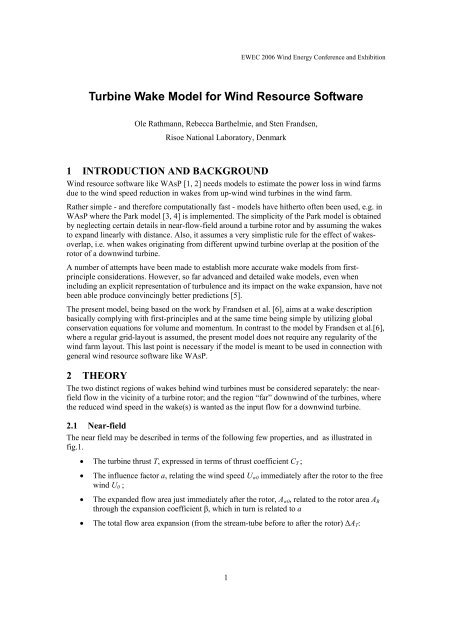
EWEC 2006 Wind Energy Conference and Exhibition
Turbine Wake Model for Wind Resource Software
Ole Rathmann, Rebecca Barthelmie, and Sten Frandsen,
Risoe National Laboratory, Denmark
1 INTRODUCTION AND BACKGROUND
Wind resource software like WAsP [1, 2] needs models to estimate the power loss in wind farms
due to the wind speed reduction in wakes from up-wind wind turbines in the wind farm.
Rather simple - and therefore computationally fast - models have hitherto often been used, e.g. in
WAsP where the Park model [3, 4] is implemented. The simplicity of the Park model is obtained
by neglecting certain details in near-flow-field around a turbine rotor and by assuming the wakes
to expand linearly with distance. Also, it assumes a very simplistic rule for the effect of wakesoverlap,
i.e. when wakes originating from different upwind turbine overlap at the position of the
rotor of a downwind turbine.
A number of attempts have been made to establish more accurate wake models from firstprinciple
considerations. However, so far advanced and detailed wake models, even when
including an explicit representation of turbulence and its impact on the wake expansion, have not
been able produce convincingly better predictions [5].
The present model, being based on the work by Frandsen et al. [6], aims at a wake description
basically complying with first-principles and at the same time being simple by utilizing global
conservation equations for volume and momentum. In contrast to the model by Frandsen et al.[6],
where a regular grid-layout is assumed, the present model does not require any regularity of the
wind farm layout. This last point is necessary if the model is meant to be used in connection with
general wind resource software like WAsP.
2 THEORY
The two distinct regions of wakes behind wind turbines must be considered separately: the nearfield
flow in the vicinity of a turbine rotor; and the region “far” downwind of the turbines, where
the reduced wind speed in the wake(s) is wanted as the input flow for a downwind turbine.
2.1 Near-field
The near field may be described in terms of the following few properties, and as illustrated in
fig.1.
• The turbine thrust T, expressed in terms of thrust coefficient C T ;
• The influence factor a, relating the wind speed U w0 immediately after the rotor to the free
wind U 0 ;
• The expanded flow area just immediately after the rotor, A w0 , related to the rotor area A R
through the expansion coefficient β, which in turn is related to a
• The total flow area expansion (from the stream-tube before to after the rotor) ΔA T :
1

EWEC 2006 Wind Energy Conference and Exhibition
0.75
0.5
T
= ρ C U (1)
1 2
2 T 0
0.25
0
A R
T
A w0
U
= (1 − a)
U (2); a= 1− 1− CT
(3)
w0 0
-0.25
U 0
U w0
A
w0
= β A (4)
R
1−
1 2 a
β=
1−
a
(5)
-0.5
-0.75
-2 -1 0 1 2
Δ A = Aaβ (6)
T
R
Figure 1. The near-field flow around a wind-turbine rotor.
2.2 The far-field
As illustrated in fig.2 one applies a cylindrical control volume aligned with the wind direction,
containing all relevant turbines, and sufficiently wide, that one has vanishing speed deficit in the
wind direction at the cylindrical surface.
U 0
U w
(y, z)
A
Figure 2. Cylindrical control volume around a set of turbines. In fact, the control volume should
include a cut-off at the ground level, but for graphical reasons this has been left out in the figure.
By combining the volume and momentum balance equations for the control volume one finds that
the flow field U w (y,z) at some downwind position must fulfill the following equation:
1
∑ Ti = ( , )( 0
− ( , ))
ρ
∫∫ U
A
w
y z U Uw
y z dydz (7)
i
or expressed in terms of the relative speed deficit δ≡
U
w
−U
U
0
0
(8):
2

EWEC 2006 Wind Energy Conference and Exhibition
1
2 ∑Ti
= δ( , )( 1 −δ( , ))
ρ
∫∫ y z y z dydz (9)
U
A
0 i
Here the integration (y,z) is over the cross section of the exit area of the control volume.
Frandsen [6] pointed out, that for a single wake one does not lose any essentials in the wake
description by assuming a top-hat wake speed profile, although in reality the profile is probably
Gaussian-like. We have adopted this idea and assume that within the wake boundary the wind
speed deficit is constant, only depending on the downwind distance from the rotor from which it
originates. We extended this assumption a bit more by also assuming the corresponding flow
profile for a composite wake (consisting of a number of wakes originating from different upwind
turbines): that the speed deficit distribution is mosaic-like, i.e. constant within each “tile” of the
mosaic. This concept will be elaborated on in more detail below.
2.3 Influence of turbulence.
An explicit description of the interaction of the turbulence field and the wake expansion is
believed to be possible, but it would require the establishment of a balance equation also for the
turbulent kinetic energy. It is possible to set up such a balance equation where the turbine power
and thrust determines the source terms at the turbine. However, such a balance equation will also
involve the dissipation of kinetic energy, and presently the required relationship between mean
flow, turbulence and turbulent dissipation within a wake is missing. Thus, it is not possible to fit
an explicit treatment of turbulence within the scope of a simple wake model based on global
balance equations. Instead the intention is to find out, how the wake expansion parameter(s) in
the model described below can be made to depend on the thrust coefficient (viz. turbulence) and
on the presence of interacting wakes.
3 MODEL
The wake-model consists of a sub-model for the downwind expansion of the wake, and a
procedure to find the wind speed distribution in the wake at some position, the latter both in the
case of the wake from a single turbine and in the case of a composite wake, consisting of a
number of overlapping single wakes. For the composite wake, a procedure for finding the full
“mosaic-tiles” speed distribution has been investigated, but a final solution procedure has not yet
been established. Consequently, this mosaic-tiles sub-model is only sketched below. Instead, we
have concentrated on the testing of a semi-linear approximation to the basic balance equation (9).
3.1 Wake expansion
Frandsen [6] originally proposed:
1/ k
⎡
k /2 x ⎤
Dw( x)
= DR
⎢β +α ⎥ with the expansion exponent 1/k = 1/2.
⎣ DR
⎦
However, in a recent work, Barthelmie, Frandsen et al. [7] found experimental evidence from the
Middelgrunden Wind Farm (see later) that the wake diameter measured far downwind tends to
zero when extrapolated back to its originating turbine (x=0), and not to D . A value of α=0.7
seemed to represent the measured data well. A modified form of the wake-expansion equation
was therefore was adopted to comply with this finding while still ensuring that the wake has the
right initial diameter corresponding to eq.(4), and still using k=2:
⎡ x ⎤
Dw( x) = DR
max ⎢β,
α ⎥
⎣ DR
⎦
1/2
(10),
3
β 1 2
R

EWEC 2006 Wind Energy Conference and Exhibition
The wake area is thus:
π
A ( ) ( ( )) 2
w
x = Dw x − ACut − off
(11)
4
where the last terms takes cut-off into account if the wake hits the ground surface.
Now, each time a wake passes a turbine enshrouded within it, it must experience an expansion
corresponding to the stream tube area expansion, ΔA T , ( eq.(6)). To take this into account we have
modified the wake diameter model further as
1/2
⎡ x ⎤
Dw( x) = DR
max ⎢β,
Γ+α ⎥ (12)
⎣ DR
⎦
Here Γ is a dimensionless number, with a value of zero at x=0, and increasing in jumps every
time a turbine is passed as
A ( x, Γ+ΔΓ) −A ( x, Γ ) =Δ A (13)
w w T
The work by Frandsen et al. [6] indicates that the expansion coefficient α should vary with the
thrust coefficient – in fact the indications go that it should be proportionally to it. However, in the
present work the coefficient α is treated as a constant model parameter.
3.2 Mosaic-tiles model
The concept of the mosaic speed deficit distribution is illustrated in fig.3. For a mosaic wake
speed distribution the balance equation (9) takes the rather complicated form:
1
n
n
T = A δ (1 −δ ) (14)
2 ∑ i
( k) ( k) ( k)
U 1 1 ( k )
0 i =
∑∑
ρ J J J
k = J
A 1
A 12
A 123
Wake 1 A 1
A 123
Wake 2
A 12
Wake 1
Wake 2
Wake 3
Wake 3
A 13
Affected rotor
Affected rotor
Ground
Ground
Figure 3. Examples of overlapping wake “mosaic-tiles” configurations.
Here J (k) denotes a tile associated with a certain sub-set of k wakes, and A and δ indexed with this
symbol denotes the tile area and the relative speed deficit within the tile. E.g., when considering
n=3 wakes, J (1) can take the values [1] , [2] and [3], while J (2) may take the values [1,2], [1,3],
[2,3].
4

EWEC 2006 Wind Energy Conference and Exhibition
3.3 Semi-linear model.
In wake calculations, for a certain downwind turbine rotor, the relevant property is the mean
value of the speed deficit over the rotor-plane area A RD :
1
A
= ∫∫ δ( y, zdydz )
(15)
RD
A
ARD
RD
Now, the semi-linear model is based on the observation that for small speed deficits, δ«1, the total
balance equation is linear in δ. This means that the contributions to the averaging integral from
the different upwind turbines are additive in the sense, that one may consider the effect of each
upwind turbine by itself, and then finally add up these contributions. This leads to the simple
linear approximation:
A
() i
1 [ Aw ( Δxi,
D) ∩ARD]
RD
A
≈ T
RD 2 ( i)
i
ρ U0 i Aw ( Δ xi,
D)
∑ (16)
() i
Here [ Aw
∩ A
RD]
indicates the overlapping area between the cross sectional area of wake no “i”
and the area A RD of the considered rotor, while Δx i,D is the downwind distance from the turbine
from which wake “i” originates.
In order to get the exact solution of the total balance equation in case of only a single wake
enshrouding entirely the downwind rotor, while having the same solution for multiple wakes in
the limit of small speed deficits, we adopt the following approximation to be used in the semilinear
model:
A
() i
1 [ Aw ( Δxi,
D) ∩ARD]
RD
A
(1 − )
RD
A
≈ T
RD
2 ( i)
i
ρ U0 i Aw ( Δ xi,
D)
∑ (17)
4 COMPARISON OF SEMI-LINEAR MODEL WITH OFF-SHORE
WIND FARM DATA
The wake model has been tested against accessible wind farm data. As a basis, for the wake
expansion coefficient a value of α =0.7 was used. However, as indicated in the figures, the
parameter was in some cases varied to see if better agreement with data could be obtained in this
way.
4.1 Middelgrunden Wind Farm data
Model predictions were compared to measured wind data from the Middelgrunden off-shore wind
farm just east of Copenhagen. Two southerly wind directions were considered. The first direction
(173°) was selected to be along the connection line between the two middle turbines, WT10 and
WT11, to get maximum wake effect in the middle of the wind farm. The second one (186°) was
selected to be along the connection line between the two southernmost turbines – WT20 and
WT19 - to get maximum wake effect at the latter. These situations are both indicated in the figure
4. The actual wind directions were measured by the yawing angle of the southern-most turbine
(WT20), while the wind speeds were deduced from the turbine power productions.
5

EWEC 2006 Wind Energy Conference and Exhibition
6180
Northing (km)
6179.5
6179
6178.5
6178
6177.5
6177
6176.5
6176
WT1
WT2
WT3
WT4
WT5
WT6
WT7
WT8
WT9
WT10
WT11
WT12
WT13
WT14
WT15
WT16
WT17
WT18
WT19
WT20
6175.5
186 deg.
173 deg.
6175
726 727 728 729 730 731 732
Easting (km)
Figure 4. “Middelgrunden Wind Farm” layout, with the Copenhagen shore-line indicated.
The wind farm consists of 20 Bonus 2MW turbines with a rotor diameter of 76 m and a hub
height of 67m. The spacing is about 2.4 rotor diameters. The arrows indicate the two wind
directions investigated.
Rel. Wind speed
1.1
1
0.9
0.8
0.7
0.6
0.5
0.4
Alfa=0.7
Meas.
0 10 20 30 40 50
Rel. Downwind Distance
MG_173_9
Free wind speed:
9 m/s ± 0.5 m/s
(62 sets of data)
Figure 5. Wind direction 173°±1°. Relative distance in rotor-diameters.
6

EWEC 2006 Wind Energy Conference and Exhibition
Relative Wind Speed
1.1
1
0.9
0.8
0.7
0.6
0.5
Alfa=0.7
Meas.
Free wind speed:
6 m/s ± 0.5 m/s
(48 sets of data)
0.4
0 20 40
Relative wind speed
1.1
1
0.9
0.8
0.7
0.6
0.5
Alfa=0.7
Meas.
Free wind speed:
9 m/s ± 0.5 m/s
(37 sets of data)
Relative Wind Speed
0.4
0 20 40
1.1
1
0.9
0.8
0.7
Alfa=0.7
0.6
Meas.
0.5
Alfa=0.6
0.4
0 20 40
Rel. Downwind Distance
MG 186 12
Free wind speed:
12 m/s ± 0.5 m/s
(7 sets of data)
Figure 6. Wind direction 186°±1°. Relative distance in rotor-diameters.
7

EWEC 2006 Wind Energy Conference and Exhibition
1.100
1.000
Alfa=0.7
Meas
Free wind speed:
Relative wind speed
0.900
0.800
0.700
0.600
6 m/s ± 0.5 m/s
0.500
1.1
155 165 175 185 195 205 215
Relative Wind Speed
1
0.9
0.8
0.7
0.6
Alfa=0.7
Meas
Free wind speed:
9 m/s ± 0.5 m/s
Relative Wind Speed
0.5
155 165 175 185 195 205 215
1.100
1.000
0.900
0.800
0.700
0.600
Alfa=0.7
Meas
Alfa=0.6
Alfa=0.5
Free wind speed:
12 m/s ± 0.5 m/s
0.500
155 165 175 185 195 205 215
Wind Direction
MG Dir 12
Figure 7. Wake dependence on southern wind direction of second turbine from South (WT19).
8

EWEC 2006 Wind Energy Conference and Exhibition
4.2 Horns Rev Wind Farm data
Model predictions were compared to measured wind data from the Horns Rev wind farm in the
North Sea West of Esbjerg (see figure 8). Two wind directions were considered, both of which
were selected to be along the lines of the wind farm to get the maximum wake effect: from due
West (270°) and from about South-East (222°). The wind directions in relation to the wind farm
layout is also shown in the figure. The actual wind direction was measured at a monitoring mast,
while the wind speed was deduced from the turbine power production.
6152
WT01
WT11
WT21
WT31
WT41
WT51
WT61
WT71
WT81
WT91
6151
WT02
WT12
WT22
WT32
WT42
WT52
WT62
WT72
WT82
WT92
WT03
WT13
WT23
WT33
WT43
WT53
WT63
WT73
WT83
WT93
Northing (km)
6150
270 deg.
WT04
WT05
WT14
WT15
WT24
WT25
WT34
WT35
WT44
WT45
WT54
WT55
WT64
WT65
WT74
WT75
WT84
WT85
WT94
WT95
6149
WT06
WT16
WT26
WT36
WT46
WT56
WT66
WT76
WT86
WT96
WT07
WT17
WT27
WT37
WT47
WT57
WT67
WT77
WT87
WT97
6148
WT08
WT18
WT28
WT38
WT48
WT58
WT68
WT78
WT88
WT98
222 deg.
6147
423 424 425 426 427 428 429 430
Easting (km)
Figure 8 The “Horns Rev Wind Farm” layout.
The wind farm consists of 80 V80 Vestas 2MW-turbines with a rotor diameter of 80m and a hub
height of 70m. The spacing is about 7 rotor diameters.
The arrows indicate the two wind directions investigated as well as the turbine lines, the data
from which have been used in the comparison.
9

EWEC 2006 Wind Energy Conference and Exhibition
Relative Speed
1.1
1
0.9
0.8
0.7
0.6
0.5
0.4
Alfa=0.7
Meas.
Alfa=1.0
0 10 20 30 40 50 60
Free wind speed:
9 m/s ± 0.5 m/s
(9 sets of data)
1.1
1
Free wind speed:
Relative wind speed
0.9
0.8
0.7
0.6
0.5
0.4
Alfa=0.7
Meas.
Alfa=0.5
0 10 20 30 40 50 60
12 m/s ± 0.5 m/s
(5 sets of data)
Rel. Downwind Distance
(HR 270 12)
Figure 9. Wind direction 270°±1°. Relative distance in rotor-diameters along W-E turbine line #4.
10

EWEC 2006 Wind Energy Conference and Exhibition
1.1
Free wind speed:
1
Relative Speed
0.9
0.8
0.7
0.6
Alfa=0.7
Meas.
Alfa=0.5
9 m/s ± 1 m/s
(56 sets of data)
0.5
0.4
0 20 40 60
Rel. Downwind Distance
Figure 10. Wind direction 222°±2°. Relative distance in rotor-diameters along diagonal line #7.
5 DISCUSSION OF MODEL COMPARISON WITH DATA
From the comparisons of the model prediction with the wind farm data the following points were
observed:
• The wind speed deficit at the first wake-effected turbine is generally predicted well;
• The wake width is generally predicted well;
• For positions with strong overlapping effects the speed deficit is mostly overpredicted, but
underpredictions are also seen (the Horns Rev wind farm). Variations in the α-value indicate
that improper modeling of the wake expansion is the cause.
6 CONCLUSION
The establishment of the semi-linear wake model, and the predictions made with it in comparison
with accessible data from wind farms have lead to the following conclusions regarding the further
development of the model:
• The proposed semi-linear wake model is able to treat wind farms of irregular lay-out;
• In the present version, the speed deficits are predicted qualitatively well, but the accuracy has
yet to be improved;
• The wake expansion coefficient for the wake from a certain turbine should be allowed to vary
with the thrust coefficient and in response to the presence of other wake(s) overlapping with
it. Further, at least for the wake originating from the first turbine in a line, it should be tested
whether a wake expansion exponent of 1/k = 1/3 (also considered by Frandsen et al. [6])
could give a better agreement with observation data.
• The “mosaic-tile” wake model should be further investigated, and if possible it should be
implemented with the aim of getting improved wake speed deficit predictions.
11

EWEC 2006 Wind Energy Conference and Exhibition
7 ACKNOWLEDMENTS
This work has in part been financed by the Danish Public Service Obligation (PSO) funds (F&U
4103). Data from Middelgrunden wind farm were kindly provided by Københavns Miljø- og
Energikontor, while data from Horns Rev wind farm were provided by Elsam Engineering.
8 REFERENCES
[1] I.Troen, E.L. Petersen: European Wind Atlas. Risø National Laboratory 1989.
[2] N.G.Mortensen, D.N.Heathfield, L.Myllerup, L.Landberg, O.Rathmann, I.Troen and
E.L.Petersen: Getting Started With WAsP8. Risø National Laboratory 2003 (Risø-I-
1950(EN) ).
[3] N.O.Jensen, A Note on Wind Generator Interaction, Risoe National Laboratory 1983.
(Risoe-M-2411)
[4] I. Katic, J. Højstrup and N.O.Jensen, A Simple Model for Cluster Efficiency. Proceedings of
European Wind Energy Conference and Exhibition, Rome, 1986; 407-410.
[5] R.J.L. Barthelmie et al., Comparison of Wake Model Simulations with Off-shore Wind
Turbine Wake Profiles Measured by Sodar. Journal of Atmospheric and Oceanic
Technology. In press.
[6] S. Frandsen et al., Analytical Modeling of Wind speed Deficit in Large Offshore Wind
Farms, Wind Energy 9 (2006).
[7] R.J.Barthelmie, S.T.Frandsen, P.-E.Rethore, M.Mechali, S.C.Pryor, L.Jensen and
P.Sørensen, Modelling and Measurements of Offshore Wakes. To be presented at the
Owemes 2006 Conference, 20-22 April, Citavecchia, Italy.
12