Gernot Hoffmann Windowed Sinc Interpolation
Gernot Hoffmann Windowed Sinc Interpolation
Gernot Hoffmann Windowed Sinc Interpolation

Create successful ePaper yourself
Turn your PDF publications into a flip-book with our unique Google optimized e-Paper software.
<strong>Gernot</strong> <strong>Hoffmann</strong><br />
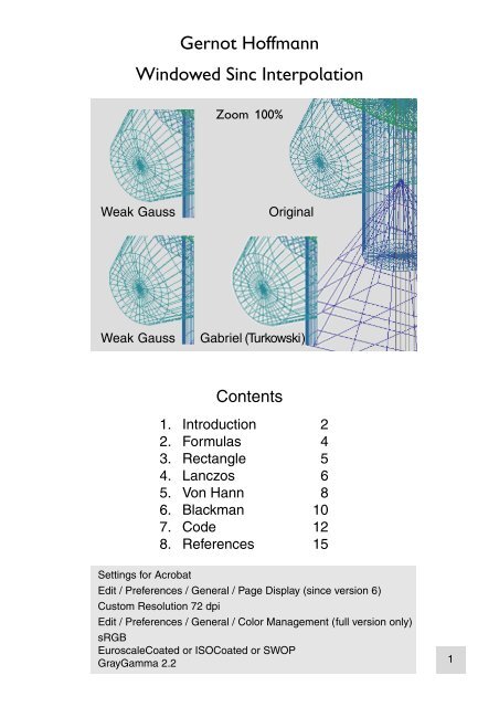
<strong>Windowed</strong> <strong>Sinc</strong> <strong>Interpolation</strong><br />
Zoom 100%<br />
Weak Gauss Original<br />
Weak Gauss Gabriel (Turkowski)<br />
Contents<br />
1. Introduction 2<br />
2. Formulas 4<br />
3. Rectangle 5<br />
4. Lanczos 6<br />
5. Von Hann 8<br />
6. Blackman 10<br />
7. Code 12<br />
8. References 15<br />
Settings for Acrobat<br />
Edit / Preferences / General / Page Display (since version 6)<br />
Custom Resolution 72 dpi<br />
Edit / Preferences / General / Color Management (full version only)<br />
sRGB<br />
EuroscaleCoated or ISOCoated or SWOP<br />
GrayGamma 2.2<br />
1
<strong>Windowed</strong> <strong>Sinc</strong> <strong>Interpolation</strong><br />
1.1 Introduction<br />
<strong>Interpolation</strong> in images can be done by many methods. Excellent references<br />
are Thévenaz et.al. [1] and Meijering [2] .<br />
In actual discussions the Lanczos interpolation is often favoured. Lanczos<br />
belongs to the so-called ’<strong>Windowed</strong> <strong>Sinc</strong>’ methods.<br />
The <strong>Sinc</strong> function is the ideal reconstruction filter (Whittaker cardinal function)<br />
for band-limited data streams of infinite length [3], [4] .<br />
Images are generally not band-limited, because single pixel lines, steps,<br />
hairs and grass generate a considerable amount of Nyquist frequencies,<br />
which cannot be handled correctly by any digital filter.<br />
Let us assume, an image with alternating vertical black and white lines is<br />
scanned in horizontal direction. We get a DC value, and in the AC part the<br />
lowest frequency is the Nyquist frequency, which is half the pixel clock<br />
frequency.<br />
Turkowsky [5] shows Bode plots, gain versus frequency. Without step responses,<br />
the frequency domain information is often misleading.<br />
The frequency axis notation is not understandable. These curves are symmetrical<br />
with respect to the Nyquist frequency.<br />
Therefore the end of the frequency axis should be either the Nyquist frequency<br />
at 0.5 or the sampling frequency at 1.0 .<br />
In this document we show interpolated step samples and interpolated oscillation<br />
samples. The oscillations are band-limited.<br />
Descriptions are in terms of signal processing.<br />
Sample period: T<br />
Effective length of the truncated sinc function: -nT...nT<br />
Rectangle Window n=5 Overshoot, ringing, DC error for steps<br />
Lanczos Window n=2, n=3 Overshoot, DC error for steps<br />
Von Hann Window n=2, n=3 Overshoot, DC error for steps<br />
Lanczos and von Hann are very similar. Overshoots will cause halos at sharp<br />
edges. They require also clipping.<br />
2
<strong>Windowed</strong> <strong>Sinc</strong> <strong>Interpolation</strong><br />
1. 2 Introduction<br />
Actually, this paper describes reconstruction. This is not exactly the same as<br />
filtering.<br />
8/16<br />
5/16<br />
0 -1/16<br />
0 1 2 3<br />
The curves are symmetrical. The right half is shown, the left side has to be<br />
mirrored.<br />
Reconstruction uses the whole infinite or truncated sinc function (blue) or<br />
the finite windowed sinc function (red).<br />
Filtering uses a finite number of weight factors from the windowed curve (red<br />
dots) in a Finite Impulse Response filter (FIR).<br />
Often we find some rounding to rational integer values. Here as an example<br />
(above) the Gabriel filter [5], which uses a 7x7 kernel with many zeros.<br />
A correctly designed FIR filter does not generate DC errors, opposed to reconstruction.<br />
Once the sinc function is windowed, then we have exactly one correct reconstruction<br />
algorithm.<br />
On the other hand we can build an arbitrary number of FIR filters of different<br />
orders, taking more or less values from the windowed sinc function. This is<br />
similar to taking values from a Gaussian bell.<br />
These considerations lead to the question, whether an FIR filter, based on<br />
windowed sinc, has any close relation to the ideal reconstruction sinc function.<br />
3
sin( pt/<br />
T)<br />
fs( t) = sin c( pt/<br />
T)<br />
=<br />
pt/<br />
T<br />
Whittaker reconstruction, valid for n Æ•<br />
sin[ p(<br />
t-kT) / T]<br />
ff() t = Â fk<br />
◊<br />
p(<br />
t-kT)/ T<br />
f () t =<br />
f<br />
n<br />
k=-n n<br />
sin[ p Í- t kTÍ/ T]<br />
 fk<br />
◊<br />
p Í- t kTÍ/ T<br />
k=-n Rectangle window function, finite n<br />
fw( t)=<br />
n = 5<br />
Ï<br />
Ì<br />
Ó<br />
1<br />
0<br />
-nT £ t £ + nT<br />
Else<br />
Rectangle 5<br />
Lanczos<br />
window function, finite n<br />
Ïsin(<br />
pt/ nT)/( pt/ nT)<br />
-nT £ t £+ nT<br />
fw( t)<br />
= Ì<br />
Ó 0<br />
Else<br />
n<br />
n<br />
=<br />
=<br />
2<br />
3<br />
Lanczos 2<br />
Lanczos 3<br />
Von Hann window function,<br />
finite n<br />
<strong>Windowed</strong> <strong>Sinc</strong> <strong>Interpolation</strong><br />
2.1 Formulas<br />
Ï05<br />
. [ 1+<br />
cos( pt/ nT)] -nT £ t £ + nT ¸<br />
fw( t)<br />
= Ì<br />
˝˛<br />
Ó 0<br />
Else<br />
n = 2<br />
n = 3<br />
Von Hann 2<br />
Von Hann 3<br />
¸<br />
˝<br />
˛<br />
Blackman window function, finite n<br />
¸<br />
˝<br />
˛<br />
t<br />
f () t<br />
u<br />
f () t<br />
s<br />
Independent variable, time<br />
Function<br />
<strong>Sinc</strong> function<br />
f () t Window function<br />
f () t <strong>Windowed</strong> sinc function<br />
f<br />
w<br />
v<br />
k<br />
f () t<br />
Ï042<br />
. + 05 . cos( pt/ nT) +0.08cos(2pt/ nT) -nT £ t £ + nT<br />
fw( t)<br />
= Ì<br />
Ó 0<br />
Else<br />
n = 2 Blackman<br />
n = 3 Blackman<br />
2<br />
3<br />
Whittaker reconstruction, windowed sinc, finite n<br />
K= ( t divT-n) ◊T<br />
n<br />
sin[ p Í- t KÍ/ T]<br />
ff() t = Â fu( K)<br />
◊fw( t-K) ◊<br />
p Í- t KÍ/ T<br />
k=-n<br />
Actual implementation in the procedure DoFilt<br />
f<br />
T<br />
Sampled<br />
function f = f ( t )<br />
Interpolated function<br />
Sample period<br />
k u k<br />
n Effective length of filter -nT...nT<br />
In the examples the sampling time T<br />
is given in ‘units’ (10 units or 40 units).<br />
The period of the damped oscillation<br />
has the length 200 units.<br />
The scale for t in the upper diagram<br />
(<strong>Sinc</strong>) is different to the scale in the<br />
other diagrams (Steps, Oscillation).<br />
¸<br />
˝<br />
˛<br />
4
<strong>Windowed</strong> <strong>Sinc</strong> <strong>Interpolation</strong><br />
3.1 Rectangle Window<br />
<strong>Sinc</strong> / Window / <strong>Windowed</strong> <strong>Sinc</strong><br />
<strong>Sinc</strong> / Window / <strong>Windowed</strong> <strong>Sinc</strong><br />
Rectangle 5, T=40 units<br />
Sampled Steps / Filtered Steps<br />
Sampled Oscillation / Filtered Oscillation<br />
Rectangle 5, T=10 units<br />
Sampled Steps / Filtered Steps<br />
Sampled Oscillation / Filtered Oscillation<br />
5
<strong>Windowed</strong> <strong>Sinc</strong> <strong>Interpolation</strong><br />
4.1 Lanczos Window<br />
<strong>Sinc</strong> / Window / <strong>Windowed</strong> <strong>Sinc</strong><br />
<strong>Sinc</strong> / Window / <strong>Windowed</strong> <strong>Sinc</strong><br />
Lanczos 2, T=40 units<br />
Sampled Steps / Filtered Steps<br />
Sampled Oscillation / Filtered Oscillation<br />
Lanczos 3, T=40 units<br />
Sampled Steps / Filtered Steps<br />
Sampled Oscillation / Filtered Oscillation<br />
6
<strong>Windowed</strong> <strong>Sinc</strong> <strong>Interpolation</strong><br />
4.2 Lanczos Window<br />
<strong>Sinc</strong> / Window / <strong>Windowed</strong> <strong>Sinc</strong><br />
<strong>Sinc</strong> / Window / <strong>Windowed</strong> <strong>Sinc</strong><br />
Lanczos 2, T=10 units<br />
Sampled Steps / Filtered Steps<br />
Sampled Oscillation / Filtered Oscillation<br />
Lanczos 3, T=10 units<br />
Sampled Steps / Filtered Steps<br />
Sampled Oscillation / Filtered Oscillation<br />
Dot distance T<br />
Dot distance T<br />
Dot distance T<br />
Dot distance T<br />
7
<strong>Windowed</strong> <strong>Sinc</strong> <strong>Interpolation</strong><br />
5.1 Von Hann Window<br />
<strong>Sinc</strong> / Window / <strong>Windowed</strong> <strong>Sinc</strong><br />
<strong>Sinc</strong> / Window / <strong>Windowed</strong> <strong>Sinc</strong><br />
von Hann 2, T=40 units<br />
Sampled Steps / Filtered Steps<br />
Sampled Oscillation / Filtered Oscillation<br />
von Hann 3, T=40 units<br />
Sampled Steps / Filtered Steps<br />
Sampled Oscillation / Filtered Oscillation<br />
8
<strong>Windowed</strong> <strong>Sinc</strong> <strong>Interpolation</strong><br />
5.2 Von Hann Window<br />
<strong>Sinc</strong> / Window / <strong>Windowed</strong> <strong>Sinc</strong><br />
<strong>Sinc</strong> / Window / <strong>Windowed</strong> <strong>Sinc</strong><br />
von Hann 2, T=10 units<br />
Sampled Steps / Filtered Steps<br />
Sampled Oscillation / Filtered Oscillation<br />
von Hann 3, T=10 units<br />
Sampled Steps / Filtered Steps<br />
Sampled Oscillation / Filtered Oscillation<br />
Dot distance T<br />
Dot distance T<br />
Dot distance T<br />
Dot distance T<br />
9
<strong>Windowed</strong> <strong>Sinc</strong> <strong>Interpolation</strong><br />
6.1 Blackman Window<br />
<strong>Sinc</strong> / Window / <strong>Windowed</strong> <strong>Sinc</strong><br />
<strong>Sinc</strong> / Window / <strong>Windowed</strong> <strong>Sinc</strong><br />
Blackman 2, T=40 units<br />
Sampled Steps / Filtered Steps<br />
Sampled Oscillation / Filtered Oscillation<br />
Blackman 3, T=40 units<br />
Sampled Steps / Filtered Steps<br />
Sampled Oscillation / Filtered Oscillation<br />
10
<strong>Windowed</strong> <strong>Sinc</strong> <strong>Interpolation</strong><br />
6.2 Blackman Window<br />
<strong>Sinc</strong> / Window / <strong>Windowed</strong> <strong>Sinc</strong><br />
<strong>Sinc</strong> / Window / <strong>Windowed</strong> <strong>Sinc</strong><br />
Blackman 2, T=10 units<br />
Sampled Steps / Filtered Steps<br />
Sampled Oscillation / Filtered Oscillation<br />
Blackman 3, T=10 units<br />
Sampled Steps / Filtered Steps<br />
Sampled Oscillation / Filtered Oscillation<br />
11
<strong>Windowed</strong> <strong>Sinc</strong> <strong>Interpolation</strong><br />
7.1 Code<br />
Const M = 1000; { For Function, x-pixels }<br />
sc = 150; { Amplitude y-pixels }<br />
x0 = 100; { x-offset }<br />
Var fu,ff: Array[0..M] Of Double; { Function, Filtered Function }<br />
fs,fv: Array[0..M] Of Double; { <strong>Sinc</strong>, <strong>Windowed</strong> <strong>Sinc</strong> }<br />
ti,t1,t2,y0,y1,y2 : Integer;<br />
T,Tw,N,sel,dt: Integer;<br />
AutoSave : Boolean;<br />
ImagName : String;<br />
FName : String[16];<br />
pal,col : Byte;<br />
Procedure FillF (sel: Integer);<br />
Var a: Double; na,nb,nc,k: Integer;<br />
Begin<br />
Case sel of<br />
1: Begin<br />
na:= M Div 4; nb:= 2*na; nc:= 3*na;<br />
For ti:=0 to na Do fu[ti]:= 0;<br />
For ti:=na+1 to nb Do fu[ti]:=-1;<br />
For ti:=nb+1 to nc Do fu[ti]:=+1;<br />
For ti:=nc+1 to M Do fu[ti]:= 0;<br />
End;<br />
2: Begin<br />
For ti:=0 to M Do fu[ti]:=exp(-ti/300)*sic(pi*ti/100);<br />
End;<br />
3: Begin { <strong>Sinc</strong> }<br />
fs[0] :=1;<br />
For ti:=1 to M Do<br />
Begin<br />
a:=pi*ti/T;<br />
fs[ti]:=sic(a)/a;<br />
End;<br />
End;<br />
10:Begin { Rectangle <strong>Windowed</strong> <strong>Sinc</strong> }<br />
fv[0] :=1;<br />
For ti:=1 to M Do fv[ti]:=0;<br />
For ti:=1 to Tw Do { Tw=5*T }<br />
Begin<br />
fv[ti]:=fs[ti];<br />
End;<br />
End;<br />
11:Begin { Lanczos <strong>Windowed</strong> <strong>Sinc</strong> }<br />
fv[0] :=1;<br />
For ti:=1 to M Do fv[ti]:=0;<br />
For ti:=1 to Tw Do<br />
Begin<br />
a:=pi*ti/Tw; { Tw=(2-3)*T }<br />
fv[ti]:=fs[ti]*sic(a)/a;<br />
End;<br />
End;<br />
End;<br />
12
<strong>Windowed</strong> <strong>Sinc</strong> <strong>Interpolation</strong><br />
7.2 Code<br />
12:Begin { von Hann <strong>Windowed</strong> <strong>Sinc</strong> }<br />
fv[0] :=1;<br />
For ti:=1 to M Do fv[ti]:=0;<br />
For ti:=1 to Tw Do<br />
Begin<br />
a:=pi*ti/Tw; { Tw=(2-3)*T }<br />
fv[ti]:=fs[ti]*0.5*(1+coc(a));<br />
End;<br />
End;<br />
13:Begin { Blackman <strong>Windowed</strong> <strong>Sinc</strong> }<br />
fv[0] :=1;<br />
For ti:=1 to M Do fv[ti]:=0;<br />
For ti:=1 to Tw Do<br />
Begin<br />
a:=pi*ti/Tw; { Tw=(2-3)*T }<br />
fv[ti]:=fs[ti]*(0.42+0.5*coc(a)+0.08*coc(2*a));<br />
End;<br />
End;<br />
End; { Case }<br />
End;<br />
Procedure DoFilt;<br />
Var s : Double;<br />
k,kT,a: Integer;<br />
Begin<br />
For ti:=0 to M-1 Do<br />
Begin<br />
kT:=((ti Div T)-N)*T;<br />
s:=0;<br />
For k:=-N to N Do<br />
Begin<br />
If (kT>=0) And (kT
<strong>Windowed</strong> <strong>Sinc</strong> <strong>Interpolation</strong><br />
7.3 Code<br />
Procedure DefFilt(ftype: Integer);<br />
Var txt: String[3];<br />
Begin<br />
Case ftype Of<br />
301: Begin FName:=’Rectangle-5-40';T:=40; N:=5; Tw:=N*T; sel:=10;<br />
End;<br />
303: Begin FName:=’Rectangle-5-10';T:=10; N:=5; Tw:=N*T; sel:=10;<br />
End;<br />
401: Begin FName:=’Lanczos-2-40'; T:=40; N:=2; Tw:=N*T; sel:=11;<br />
End;<br />
402: Begin FName:=’Lanczos-3-40'; T:=40; N:=3; Tw:=N*T; sel:=11;<br />
End;<br />
403: Begin FName:=’Lanczos-2-10'; T:=10; N:=2; Tw:=N*T; sel:=11;<br />
End;<br />
404: Begin FName:=’Lanczos-3-10'; T:=10; N:=3; Tw:=N*T; sel:=11;<br />
End;<br />
501: Begin FName:=’von-Hann-2-40'; T:=40; N:=2; Tw:=N*T; sel:=12;<br />
End;<br />
502: Begin FName:=’von-Hann-3-40'; T:=40; N:=3; Tw:=N*T; sel:=12;<br />
End;<br />
503: Begin FName:=’von-Hann-2-10'; T:=10; N:=2; Tw:=N*T; sel:=12;<br />
End;<br />
504: Begin FName:=’von-Hann-3-10'; T:=10; N:=3; Tw:=N*T; sel:=12;<br />
End;<br />
601: Begin FName:=’Blackman-2-40'; T:=40; N:=2; Tw:=N*T; sel:=13;<br />
End;<br />
602: Begin FName:=’Blackman-3-40'; T:=40; N:=3; Tw:=N*T; sel:=13;<br />
End;<br />
603: Begin FName:=’Blackman-2-10'; T:=10; N:=2; Tw:=N*T; sel:=13;<br />
End;<br />
604: Begin FName:=’Blackman-3-10'; T:=10; N:=3; Tw:=N*T; sel:=13;<br />
End;<br />
End; { case }<br />
End;<br />
Source code does not contain graphics procedures etc..<br />
14
<strong>Windowed</strong> <strong>Sinc</strong> <strong>Interpolation</strong><br />
8.1 References<br />
[1] PhilippeThévenaz + Thierry Blu + Michael Unser<br />
Interpolaton Revisited<br />
IEEE Transactions on Medical Imaging, Vol.19, 7.July 2000<br />
URL:<br />
[2] Erik Meijering<br />
A Chronology of <strong>Interpolation</strong>: From Ancient Astronomy to Modern Signal and<br />
Image Processing<br />
Proceedings of the IEEE, Vol.90, 3.March 2002<br />
URL:<br />
[3] Samuel D.Stearns<br />
Digitale Verarbeitung analoger Signale<br />
R.Oldenbourg Verlag München Wien, 1988<br />
[4] Elmar Schrüfer<br />
Signalverarbeitung<br />
Carl Hanser Verlag München Wien, 1990<br />
[5] Ken Turkowsky<br />
Filters for Common Resampling Tasks<br />
10.April 1990<br />
http://www.worldserver.com/turk/computergraphics/ResamplingFilters.pdf<br />
[6] <strong>Gernot</strong> <strong>Hoffmann</strong><br />
Bilinear, Biquadratic, Bicubic and Bicubic Spline <strong>Interpolation</strong><br />
http://www.fho-emden.de/~hoffmann/bicubic03042002.pdf<br />
This document<br />
http://www.fho-emden.de/~hoffmann/lanczos07112002.pdf<br />
Blackman was added January 26 / 2008<br />
<strong>Gernot</strong> <strong>Hoffmann</strong><br />
November 11 / 2002 - January 28 / 2008<br />
Website: load browser, click here 15<br />
15


![[PDF] SpieleProgrammierung](https://img.yumpu.com/6860251/1/190x135/pdf-spieleprogrammierung.jpg?quality=85)