Longitudinal Data Analysis for Social Science ... - ReStore
Longitudinal Data Analysis for Social Science ... - ReStore
Longitudinal Data Analysis for Social Science ... - ReStore

Create successful ePaper yourself
Turn your PDF publications into a flip-book with our unique Google optimized e-Paper software.
<strong>Longitudinal</strong> <strong>Data</strong> <strong>Analysis</strong> <strong>for</strong><br />
<strong>Social</strong> <strong>Science</strong> Researchers<br />
Introduction to Panel Models<br />
www.longitudinal.stir.ac.uk<br />
SIMPLE TABLE – PANEL DATA<br />
Women in their 20s in 1991 – Ten Years Later<br />
Count<br />
Marital status WAVE J * Marital status WAVE A Crosstabulation<br />
Marital status WAVE A<br />
Marital<br />
status<br />
WAVE J<br />
Total<br />
Married<br />
Living as couple<br />
Widowed<br />
Divorced<br />
Separated<br />
Never married<br />
Living as<br />
Married couple Widowed Divorced Separated Never married Total<br />
324 74 0 4 9 102 513<br />
16 33 1 5 6 44 105<br />
4 1 1 0 1 0 7<br />
36 5 0 4 9 3 57<br />
12 1 0 0 2 5 20<br />
1 18 0 0 0 85 104<br />
393 132 2 13 27 239 806<br />
BEWARE<br />
BEWARE<br />
1
• Traditionally used in social mobility work<br />
• Can be made more exotic <strong>for</strong> example by<br />
incorporating techniques from loglinear<br />
modelling (there is a large body of<br />
methodological literature in this area)<br />
Change Score<br />
• Less likely to use this approach in<br />
mainstream social science<br />
• Understanding this will help you<br />
understand the foundation of more<br />
complex panel models (especially this<br />
afternoon)<br />
Vector of explanatory<br />
variables and estimates<br />
Y i 1<br />
= β’X i1<br />
+ ε i1<br />
Outcome 1 <strong>for</strong><br />
individual i<br />
Independent<br />
identifiably<br />
distributed error<br />
2
EQUATION FOR TIME POINT 2<br />
Y i 1<br />
= β’X i1<br />
+ ε i1<br />
Vector of explanatory<br />
variables and estimates<br />
Outcome 1 <strong>for</strong><br />
individual i<br />
Independent<br />
identifiably<br />
distributed error<br />
Considered together conventional<br />
regression analysis in NOT appropriate<br />
Y i 1<br />
= β’X i1<br />
+ ε i1<br />
Y i 2<br />
= β’X i2<br />
+ ε i2<br />
Change in Score<br />
Y i 2<br />
-Y i 1<br />
= β’(X i2 -X i1 ) + (ε i2<br />
- ε i1<br />
)<br />
Here the β’ is simply a regression on the<br />
difference or change in scores.<br />
3
Women in 20s H.H. Income Month<br />
Be<strong>for</strong>e Interview (Wfihhmn)<br />
MEAN<br />
S.D.<br />
MEDIAN<br />
SKEWNESS<br />
PERCENTILES<br />
25%<br />
75%<br />
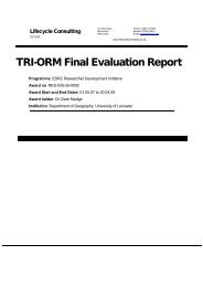
r =.679**<br />
WAVE A<br />
1793.50<br />
1210.26<br />
1566.34<br />
1.765<br />
914.43<br />
2339.39<br />
WAVE B<br />
1788.15<br />
1171.36<br />
1587.50<br />
1.404<br />
950.51<br />
2353.85<br />
A Simple Scatter Plot<br />
Household income: month be<strong>for</strong>e interview Wave B<br />
10000<br />
8000<br />
6000<br />
4000<br />
2000<br />
0<br />
-2000<br />
-2000<br />
0<br />
2000<br />
4000<br />
6000<br />
8000<br />
10000<br />
Household income: month be<strong>for</strong>e interview Wave A<br />
Change in Score<br />
Y i 2<br />
-Y i 1<br />
= β’(X i2 -X i1 ) + (ε i2<br />
- ε i1<br />
)<br />
Difference or change in scores<br />
(bfihhmn – afihhmn)<br />
Here the β’ is simply a regression on the<br />
difference or change in scores.<br />
4
Models <strong>for</strong> Multiple Measures<br />
Panel Models<br />
PID<br />
WAVE<br />
SEX<br />
AGE<br />
Y<br />
001<br />
1<br />
1<br />
20<br />
1<br />
001<br />
2<br />
1<br />
21<br />
1<br />
001<br />
3<br />
1<br />
22<br />
1<br />
001<br />
4<br />
1<br />
23<br />
0<br />
001<br />
5<br />
1<br />
24<br />
0<br />
001<br />
6<br />
1<br />
25<br />
1<br />
Models <strong>for</strong> Multiple Repeated<br />
Measures<br />
“Increasingly, I tend to think of these<br />
approaches as falling under the general<br />
umbrella of generalised linear modelling<br />
(glm). This allows me to think about<br />
longitudinal data analysis simply as an<br />
extension of more familiar statistical<br />
models from the regression family. It also<br />
helps to facilitate the interpretation of<br />
results.”<br />
5
Some Common Panel Models<br />
(STATA calls these Cross-sectional time series!)<br />
Binary Y Logit xtlogit<br />
(Probit xtprobit)<br />
Count Y Poisson xtpoisson<br />
(Neg bino xtnbreg)<br />
Continuous Y<br />
Regression xtreg<br />
Models <strong>for</strong> Multiple Measures<br />
As social scientists we are<br />
often substantively interested<br />
in whether a specific event<br />
has occurred.<br />
There<strong>for</strong>e <strong>for</strong> the next 30<br />
minutes I will mostly be<br />
concentrating on models <strong>for</strong><br />
binary outcomes<br />
6
Recurrent events are merely outcomes that can<br />
take place on a number of occasions. A simple<br />
example is unemployment measured month by<br />
month. In any given month an individual can<br />
either be employed or unemployed. If we had<br />
data <strong>for</strong> a calendar year we would have twelve<br />
discrete outcome measures (i.e. one <strong>for</strong> each<br />
month).<br />
Consider a binary outcome or<br />
two-state event<br />
0 = Event has not occurred<br />
1 = Event has occurred<br />
In the cross-sectional situation we<br />
are used to modelling this with<br />
logistic regression.<br />
UNEMPLOYMENT AND<br />
RETURNING TO WORK STUDY<br />
–<br />
A study <strong>for</strong> six months<br />
0 = Unemployed; 1 = Working<br />
7
Months<br />
1 2 3 4 5 6<br />
obs 0 0 0 0 0 0<br />
Constantly unemployed<br />
Months<br />
1 2 3 4 5 6<br />
obs 1 1 1 1 1 1<br />
Constantly employed<br />
Months<br />
1 2 3 4 5 6<br />
obs 1 0 0 0 0 0<br />
Employed in month 1<br />
then unemployed<br />
8
Months<br />
1 2 3 4 5 6<br />
obs 0 0 0 0 0 1<br />
Unemployed but gets a job in<br />
month six<br />
Here we have a binary<br />
outcome – so could we simply<br />
use logistic regression to<br />
model it?<br />
Yes and No – We need to<br />
think about this issue.<br />
POOLED CROSS-SECTIONAL LOGIT MODEL<br />
L<br />
B<br />
it<br />
( β )<br />
=<br />
[exp(<br />
β ' x<br />
1 + exp(<br />
it<br />
)]<br />
y<br />
β ' x<br />
it<br />
it<br />
)<br />
x it<br />
is a vector of explanatory variables and β is a vector of<br />
parameter estimates<br />
9
We could fit a pooled crosssectional<br />
model to our<br />
recurrent events data.<br />
This approach can be<br />
regarded as a naïve solution<br />
to our data analysis problem.<br />
We need to consider a number<br />
of issues….<br />
Months<br />
Y 1 Y 2<br />
obs 0 0<br />
Pickle’s tip - In repeated measures analysis<br />
we would require something like a ‘paired’ t test<br />
rather than an ‘independent’ t test because we<br />
can assume that Y1 and Y2 are related.<br />
10
Repeated measures data violate<br />
an important assumption of<br />
conventional regression models.<br />
The responses of an individual at<br />
different points in time will not be<br />
independent of each other.<br />
The observations are “clusters” in the individual<br />
SUBJECT<br />
Wave A Wave B Wave C Wave D Wave E<br />
REPEATED MEASURES / OBSERVATIONS<br />
Repeated measures data violate<br />
an important assumption of<br />
conventional regression models.<br />
The responses of an individual at<br />
different points in time will not be<br />
independent of each other.<br />
This problem has been overcome<br />
by the inclusion of an additional,<br />
individual-specific error term.<br />
11
L<br />
L<br />
POOLED CROSS-SECTIONAL LOGIT MODEL<br />
B<br />
it<br />
B<br />
it<br />
( β )<br />
( β ) =<br />
⎡<br />
⎢<br />
⎢⎣<br />
T<br />
i<br />
= ∫ ∏<br />
[exp(<br />
1 +<br />
β ' x<br />
exp(<br />
PANEL LOGIT MODEL (RANDOM EFFECTS MODEL)<br />
Simplified notation!!!<br />
yit<br />
[exp( β ' xit<br />
+ ε)]<br />
⎤<br />
⎥f(<br />
ε<br />
1+<br />
exp( β ' x + ε)<br />
⎥⎦<br />
t= 1<br />
it<br />
it<br />
)]<br />
y<br />
β ' x<br />
it<br />
it<br />
)<br />
) dε<br />
L<br />
B<br />
it<br />
( β )<br />
For a sequence of outcomes <strong>for</strong><br />
the i th case, the basic random<br />
effects model has the integrated<br />
(or marginal likelihood) given by<br />
the equation.<br />
⎡<br />
⎢<br />
⎢⎣<br />
T<br />
i<br />
= ∫ ∏<br />
yit<br />
[exp( β ' xit<br />
+ ε)]<br />
⎤<br />
⎥f(<br />
ε<br />
1+<br />
exp( β ' x + ε)<br />
⎥⎦<br />
t= 1<br />
it<br />
) dε<br />
The random effects model extends<br />
the pooled cross-sectional model<br />
to include a case-specific random<br />
error term this helps to account <strong>for</strong><br />
residual heterogeneity.<br />
12
Davies and Pickles (1985) have demonstrated<br />
that the failure to explicitly model the effects of<br />
residual heterogeneity may cause severe bias in<br />
parameter estimates. Using longitudinal data the<br />
effects of omitted explanatory variables can be<br />
overtly accounted <strong>for</strong> within the statistical<br />
model. This greatly improves the accuracy of<br />
the estimated effects of the explanatory<br />
variables.<br />
An simple example –<br />
Davies, Elias & Penn (1992)<br />
The relationship between a<br />
husband’s unemployment and<br />
his wife’s participation in the<br />
labour <strong>for</strong>ce<br />
13
Four waves of BHPS data<br />
Married Couples in their 20s (n=515; T=4; obs=2060)<br />
Summary in<strong>for</strong>mation…<br />
56% of women working (in paid employment)<br />
59% of women with employed husbands work<br />
23% of women with unemployed husbands work<br />
65% of women without a child under 5 work<br />
48% of women with a child under 5 work<br />
POOLED (cross-sectional) MODELS<br />
MODEL<br />
Null Model<br />
+ husband<br />
unemployed<br />
+husband u<br />
+child und 5<br />
husband u *<br />
child und 5<br />
Deviance<br />
(Log L)<br />
2830<br />
(-1415)<br />
2732<br />
(-1366)<br />
2692<br />
(-1346)<br />
2692<br />
(-1346)<br />
Change d.f.<br />
-<br />
1<br />
1<br />
1<br />
No. obs<br />
2060<br />
2060<br />
2060<br />
2060<br />
First glimpse at STATA<br />
• Models <strong>for</strong> panel data<br />
• STATA – unhelpfully calls this ‘crosssectional<br />
time-series’<br />
• xt commands suite<br />
14
STATA CODE<br />
Cross-Sectional Model<br />
Cross-Sectional Model<br />
logit y mune und5<br />
logit y mune und5, cluster (pid)<br />
POOLED MODELS<br />
Cross-sectional<br />
(pooled)<br />
Beta<br />
S.E.<br />
Cross-sectional<br />
(cluster)<br />
Beta<br />
S.E.<br />
Husband<br />
unemployed<br />
-1.49<br />
0.18<br />
-1.49<br />
0.23<br />
Child under 5<br />
-0.59<br />
0.09<br />
-0.59<br />
0.13<br />
Constant<br />
0.69<br />
0.07<br />
0.69<br />
0.11<br />
xtdes, i(pid) t(year)<br />
xtdes, i(pid) t(year)<br />
pid: 10047093, 10092986, ..., 19116969 n = 515<br />
year: 91, 92, ..., 94 T = 4<br />
Delta(year) = 1; (94-91)+1 = 4<br />
(pid*year uniquely identifies each observation)<br />
Distribution of T_i: min 5% 25% 50% 75% 95% max<br />
4 4 4 4 4 4 4<br />
Freq. Percent Cum. | Pattern<br />
---------------------------+---------<br />
515 100.00 100.00 | 1111<br />
---------------------------+---------<br />
515 100.00 | XXXX<br />
15
xtdes, i(pid) t(year)<br />
xtdes, i(pid) t(year)<br />
pid: 10047093, 10092986, ..., 19116969 n = 515<br />
year: 91, 92, ..., 94 T = 4<br />
xtdes, i(pid) t(year)<br />
Delta(year) = 1; (94-91)+1 = 4<br />
(pid*year uniquely identifies each observation)<br />
xtdes, i(pid) t(year)<br />
Distribution of T_i: min 5% 25% 50% 75% 95% max<br />
4 4 4 4 4 4 4<br />
16
xtdes, i(pid) t(year)<br />
Note: this is a<br />
balanced panel<br />
Freq. Percent Cum. | Pattern<br />
---------------------------+---------<br />
515 100.00 100.00 | 1111<br />
---------------------------+---------<br />
515 100.00 | XXXX<br />
xtdes, i(pid) t(year)<br />
xtdes, i(pid) t(year)<br />
pid: 10047093, 10092986, ..., 19116969 n = 515<br />
year: 91, 92, ..., 94 T = 4<br />
Delta(year) = 1; (94-91)+1 = 4<br />
(pid*year uniquely identifies each observation)<br />
Distribution of T_i: min 5% 25% 50% 75% 95% max<br />
4 4 4 4 4 4 4<br />
Freq. Percent Cum. | Pattern<br />
---------------------------+---------<br />
515 100.00 100.00 | 1111<br />
---------------------------+---------<br />
515 100.00 | XXXX<br />
POOLED & PANEL MODELS<br />
MODEL<br />
Pooled Model<br />
Panel Model<br />
Deviance<br />
(Log L)<br />
2692<br />
(-1346)<br />
2186<br />
(-1093)<br />
Change<br />
d.f.<br />
-<br />
1<br />
No. obs<br />
2060<br />
2060<br />
(n=515)<br />
The panel model is clearly an improvement on<br />
the pooled cross-sectional analysis. We can<br />
suspect non-independence of observations.<br />
17
FURTHER - EXPLORATION<br />
PANEL MODELS<br />
MODEL<br />
Null Model<br />
+ husband<br />
unemployed<br />
+husband u<br />
+child und 5<br />
husband u *<br />
child und 5<br />
Deviance<br />
(Log L)<br />
2218<br />
(-1109)<br />
2196<br />
(-1098)<br />
2186<br />
(-1093)<br />
2186<br />
(-1093)<br />
Change d.f.<br />
-<br />
1<br />
1<br />
1<br />
No. obs<br />
(n)<br />
2060<br />
(515)<br />
2060<br />
(515)<br />
2060<br />
(515)<br />
2060<br />
(515)<br />
COMPARISON OF MODELS<br />
Cross-sectional<br />
(pooled)<br />
Random Effects<br />
Beta<br />
S.E.<br />
Rob<br />
S.E.<br />
Beta<br />
S.E.<br />
Husband<br />
unemployed<br />
-1.49<br />
0.18<br />
0.23<br />
-.83<br />
.18<br />
Child under 5<br />
-0.59<br />
0.09<br />
0.13<br />
-.34<br />
.10<br />
Constant<br />
0.69<br />
0.07<br />
0.11<br />
.53<br />
.10<br />
18
STATA OUTPUT<br />
Random-effects logistic regression Number of obs = 2060<br />
Group variable (i): pid Number of groups = 515<br />
Random effects u_i ~ Gaussian Obs per group: min = 4<br />
avg = 4.0<br />
max = 4<br />
Wald chi2(2) = 31.73<br />
Log likelihood = -1093.3383 Prob > chi2 = 0.0000<br />
------------------------------------------------------------------------------<br />
y | Coef. Std. Err. z P>|z| [95% Conf. Interval]<br />
-------------+----------------------------------------------------------------<br />
_Imune_1 | -1.351039 .3029752 -4.46 0.000 -1.944859 -.7572184<br />
_Iund5_1 | -.5448233 .1712375 -3.18 0.001 -.8804426 -.209204<br />
_cons | .8551312 .1557051 5.49 0.000 .5499549 1.160307<br />
-------------+----------------------------------------------------------------<br />
/lnsig2u | 1.659831 .0974218 1.468888 1.850774<br />
-------------+----------------------------------------------------------------<br />
sigma_u | 2.293125 .1117002 2.084322 2.522845<br />
rho | .6151431 .0230638 .5690656 .6592439<br />
------------------------------------------------------------------------------<br />
Likelihood-ratio test of rho=0: chibar2(01) = 504.79 Prob >= chibar2 = 0.000<br />
19
Random-effects logistic regression Number of obs = 2060<br />
Group variable (i): pid Number of groups = 515<br />
Random effects u_i ~ Gaussian Obs per group: min = 4<br />
avg = 4.0<br />
max = 4<br />
Wald chi2(2) = 31.73<br />
Log likelihood = -1093.3383 Prob > chi2 = 0.0000<br />
------------------------------------------------------------------------------<br />
y | Coef. Std. Err. z P>|z| [95% Conf. Interval]<br />
-------------+----------------------------------------------------------------<br />
_Imune_1 | -1.351039 .3029752 -4.46 0.000 -1.944859 -.7572184<br />
_Iund5_1 | -.5448233 .1712375 -3.18 0.001 -.8804426 -.209204<br />
_cons | .8551312 .1557051 5.49 0.000 .5499549 1.160307<br />
-------------+----------------------------------------------------------------<br />
/lnsig2u | 1.659831 .0974218 1.468888 1.850774<br />
-------------+----------------------------------------------------------------<br />
sigma_u | 2.293125 .1117002 2.084322 2.522845<br />
rho | .6151431 .0230638 .5690656 .6592439<br />
------------------------------------------------------------------------------<br />
Likelihood-ratio test of rho=0: chibar2(01) = 504.79 Prob >= chibar2 = 0.000<br />
-------------+----------------------------------------------------------------<br />
/lnsig2u | 1.659831 .0974218 1.468888 1.850774<br />
-------------+----------------------------------------------------------------<br />
sigma_u | 2.293125 .1117002 2.084322 2.522845<br />
rho | .6151431 .0230638 .5690656 .6592439<br />
------------------------------------------------------------------------------<br />
Likelihood-ratio test of rho=0: chibar2(01) = 504.79 Prob >= chibar2 = 0.000<br />
sigma_u can be interpreted like a parameter estimate with a standard error<br />
Remember it is the root of anti log - sig2u<br />
(expσ<br />
2 )<br />
20
-------------+----------------------------------------------------------------<br />
/lnsig2u | 1.659831 .0974218 1.468888 1.850774<br />
-------------+----------------------------------------------------------------<br />
sigma_u | 2.293125 .1117002 2.084322 2.522845<br />
rho | .6151431 .0230638 .5690656 .6592439<br />
------------------------------------------------------------------------------<br />
Likelihood-ratio test of rho=0: chibar2(01) = 504.79 Prob >= chibar2 = 0.000<br />
rho = sigma_u / (sigma_u + sigma_e)<br />
rho can be appreciated as the proportion of the total<br />
variance contributed by the panel-level (i.e. subject<br />
level) variance component<br />
When rho is zero the panel-level variance<br />
component is unimportant. A likelihood ratio test is<br />
provided at the bottom of the output<br />
You can think of rho as being the (analogous)<br />
equivalent of the intra-cluster correlation (icc) in<br />
a multilevel model<br />
SUBJECT<br />
Wave A Wave B Wave C Wave D Wave E<br />
REPEATED MEASURES / OBSERVATIONS<br />
SOME CONCLUSIONS<br />
• Panel models are attractive<br />
• Extend cross-sectional (glm) models<br />
• They overcome the non-independence<br />
problem<br />
• Provide increased control <strong>for</strong> residual<br />
heterogeneity<br />
• Can be extended to provide increased control<br />
<strong>for</strong> state dependence<br />
21
Some Restrictions<br />
• Specialist software (e.g. STATA)<br />
• {Powerful computers required}<br />
• Results can be complicated to interpret<br />
• Real data often behaves badly (e.g.<br />
unbalanced panel)<br />
• Communication of results can be more<br />
tricky<br />
22