Ankle and Foot 47 - Department of Radiology - University of ...
Ankle and Foot 47 - Department of Radiology - University of ...
Ankle and Foot 47 - Department of Radiology - University of ...

You also want an ePaper? Increase the reach of your titles
YUMPU automatically turns print PDFs into web optimized ePapers that Google loves.
Ken L. Schreibman<br />
Richard Bruce<br />
<strong>Ankle</strong> <strong>and</strong> <strong>Foot</strong> <strong>47</strong><br />
This chapter is intended to serve as a practical approach to<br />
imaging the ankle <strong>and</strong> foot using computed tomography<br />
(CT) <strong>and</strong> magnetic resonance imaging (MRI). Rather than<br />
providing an exhaustive review <strong>of</strong> the literature, we illustrate<br />
the anatomic structures <strong>and</strong> common pathologic<br />
processes seen with CT <strong>and</strong> MRI scans. In addition, we have<br />
included discussions regarding the techniques for obtaining<br />
these scans, including the CT <strong>and</strong> MR protocol sheets<br />
we use daily in the <strong>Radiology</strong> <strong>Department</strong> <strong>of</strong> the <strong>University</strong><br />
<strong>of</strong> Wisconsin in Madison (UW). The most up-to-date versions<br />
<strong>of</strong> these protocol sheets are available for free download<br />
at www.schreibman.info. Throughout this chapter, we<br />
have endeavored to include references to review articles for<br />
readers who wish to explore topics in more detail. The<br />
images <strong>and</strong> content <strong>of</strong> this chapter are based on Dr.<br />
Schreibman’s lecture series.<br />
Anatomy<br />
• Tarsal Bones<br />
• Gross Anatomy <strong>of</strong> the Tarsal Bones 15<br />
Talus<br />
Figures <strong>47</strong>-1 through <strong>47</strong>-4 are photographs <strong>of</strong> cadaveric<br />
bones arranged to illustrate the relationships <strong>of</strong> the major<br />
tarsal bones <strong>and</strong> joints. Figure <strong>47</strong>-1 represents the bones<br />
we typically cover when scanning the distal tibia/ankle/<br />
foot. Central to all this is the talus, labeled Ta. (The label<br />
abbreviations in Fig. <strong>47</strong>-1 will be consistent throughout all<br />
figures.) Indeed, the word talus is Latin for “ankle,” indicating<br />
that early anatomists considered the talus the center <strong>of</strong><br />
the ankle. Underst<strong>and</strong>ing the articulations between the<br />
talus <strong>and</strong> the surrounding bones is the key to underst<strong>and</strong>ing<br />
the anatomy <strong>of</strong> the ankle <strong>and</strong> foot.<br />
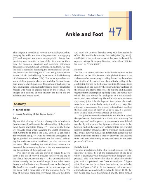
Two views <strong>of</strong> the talus are shown in Figure <strong>47</strong>-2. The<br />
dome is the broad, curved articular surface on the top <strong>of</strong><br />
the talus. (The specimen in Fig. <strong>47</strong>-2 has an osteochondral<br />
lesion centrally in the medial edge <strong>of</strong> the talar dome.<br />
Osteochondral lesions are discussed later in the chapter.)<br />
The head is the rounded process at the anterior aspect <strong>of</strong><br />
the talus, <strong>and</strong> it articulates with the navicular bone. The<br />
body <strong>of</strong> the talus comprises everything between the dome<br />
<strong>and</strong> head. The dome <strong>of</strong> the talus along with the distal ends<br />
<strong>of</strong> the tibia <strong>and</strong> fibula make up the ankle joint (Fig. <strong>47</strong>-3).<br />
(<strong>Ankle</strong> joint is the preferred name <strong>of</strong> this joint in the radiology<br />
<strong>and</strong> orthopedic surgery literature, rather than “tibiotalar<br />
joint” or “crural joint.”)<br />
Mortise<br />
The flat talar dome articulates with the flat surface at the<br />
distal end <strong>of</strong> the tibia known as the plafond. Plafond is an<br />
architectural term meaning “a ceiling formed by the underside<br />
<strong>of</strong> a floor.” In essence, the plafond is the ceiling <strong>of</strong> the<br />
ankle joint, formed by the floor <strong>of</strong> the tibia. The ankle joint<br />
is bounded on the sides by the inner articular surfaces <strong>of</strong><br />
the medial <strong>and</strong> lateral malleoli. The plafond <strong>and</strong> malleoli<br />
together form a rectangular opening called the mortise into<br />
which the talar domes fit, analogous to a mortise-<strong>and</strong>tenon<br />
joint in woodworking. The ankle mortise is a remarkably<br />
sturdy joint. Like the hip <strong>and</strong> knee joints, the ankle<br />
must bear our entire body weight with every step. But<br />
although it is common for primary osteoarthritis to affect<br />
the hips <strong>and</strong> knees <strong>of</strong> many <strong>of</strong> us as we age, it is uncommon<br />
to have primary osteoarthritis <strong>of</strong> the ankle.<br />
The joint between the distal tibia <strong>and</strong> fibula is called<br />
the syndesmosis. Syndesmosis is a Greek term meaning “to<br />
bind together,” <strong>and</strong> in general a syndesmosis joint is held<br />
together by thick connective ligaments. (Most joints in the<br />
body, including the ankle <strong>and</strong> subtalar joints, are synovial<br />
joints in that they are enclosed by a synovium-lined capsule<br />
that creates synovial fluid.) The distal fibula, just above the<br />
lateral malleolus, fits into a shallow groove in the adjacent<br />
tibia, <strong>and</strong> this relationship is best visualized in the axial<br />
plane <strong>of</strong> a CT scan.<br />
Subtalar Joint<br />
The talus articulates with the tibia from above <strong>and</strong> with the<br />
navicular in front. It is at the undersurface <strong>of</strong> the talus<br />
where it articulates with the calcaneus that things get complicated.<br />
This joint below the talus is called the subtalar<br />
joint, which is preferred over “talocalcaneal joint.” Figure<br />
<strong>47</strong>-4 illustrates the three facets that make up the subtalar<br />
joint. In Figure <strong>47</strong>-4A to D, the talus <strong>and</strong> calcaneus were<br />
attached using colored modeling clay. In Figure <strong>47</strong>-4E, the<br />
two bones have been disarticulated <strong>and</strong> the talus flipped<br />
2207<br />
Ch0<strong>47</strong>-A05375.indd 2207<br />
9/9/2008 5:33:07 PM
2208 VII Imaging <strong>of</strong> the Musculoskeletal System<br />
over, displaying the talar <strong>and</strong> calcaneal articular surfaces <strong>of</strong><br />
the posterior, middle, <strong>and</strong> anterior facets <strong>of</strong> the subtalar<br />
joint in red, blue, <strong>and</strong> green, respectively.<br />
The posterior facet is the largest <strong>and</strong> is the primary<br />
weight-bearing portion <strong>of</strong> the subtalar joint. At the anterolateral<br />
corner <strong>of</strong> the posterior facet, the talus comes to an<br />
acutely angled corner, the lateral process <strong>of</strong> the talus. When<br />
the subtalar joint experiences an extreme axial load, such<br />
as when a person falls from a height or undergoes a deceleration<br />
injury in a motor vehicle collision, the pointy<br />
lateral process <strong>of</strong> the talus acts like a wedge, splitting<br />
<strong>and</strong> fracturing the calcaneus. 13 Calcaneal fractures tend to<br />
extend into the posterior facet, <strong>and</strong> when imaging calcaneal<br />
fractures we obliquely angle our coronally reformatted<br />
CT slices to be perpendicular to the posterior facet.<br />
The middle facet is defined by the sustentaculum tali,<br />
a shelflike projection from the anteromedial portion <strong>of</strong> the<br />
calcaneus that supports the middle <strong>of</strong> the talus. Sustentaculum<br />
in Latin means “a supporting structure.” The flexor<br />
hallucis longus tendon passes under the sustentaculum<br />
tali. The middle facet <strong>of</strong> the subtalar joint is a completely<br />
separate articulation from the posterior facet. When injecting<br />
contrast (<strong>of</strong>ten mixed with anesthetic) into the posterior<br />
facet <strong>of</strong> the subtalar joint, we do not expect it to<br />
communicate with the middle facet. Across the middle<br />
facet <strong>of</strong> the subtalar joint is one <strong>of</strong> the two most common<br />
locations for tarsal coalitions to occur, the other being<br />
between the anterior process <strong>of</strong> the calcaneus <strong>and</strong> the<br />
lateral pole <strong>of</strong> the navicular.<br />
Unlike the posterior <strong>and</strong> middle facets, the anterior<br />
facet is not well defined <strong>and</strong> may even be absent. When<br />
present, the anterior facet is a smooth continuation <strong>of</strong> the<br />
middle facet, extending under the head <strong>of</strong> the talus. Directly<br />
lateral to the anterior <strong>and</strong> middle facet is the sinus tarsi, an<br />
area devoid <strong>of</strong> bone <strong>and</strong> filled primarily with fat.<br />
• Anatomic Divisions<br />
Figure <strong>47</strong>-5 is a three-dimensionally reformatted CT image<br />
showing the anatomic divisions between the tarsals <strong>and</strong><br />
metatarsals. The hindfoot consists <strong>of</strong> the talus <strong>and</strong> the calcaneus<br />
<strong>and</strong> is separated from the midfoot by the Chopart*<br />
joint, a smooth continuation between the talonavicular<br />
<strong>and</strong> calcaneocuboid joints. The midfoot consists <strong>of</strong> the<br />
other five tarsal bones, the navicular, the cuboid, <strong>and</strong> the<br />
three cuneiforms. The forefoot consists <strong>of</strong> the metatarsals<br />
<strong>and</strong> phalanges <strong>and</strong> is separated from the midfoot by the<br />
tarsometatarsal joint, also known as the Lisfranc † joint. Along<br />
Figure <strong>47</strong>-1. Gross anatomy <strong>of</strong> the tarsals <strong>and</strong> surrounding bones.<br />
Ti, tibia; Fi; fibula; Ta, talus; Ca, calcaneus; ST, sustentaculum tali;<br />
N, navicular; Cu, cuboid; 1, 2, <strong>and</strong> 3, refer respectively to the first,<br />
second, <strong>and</strong> third cuneiforms (sometimes referred to as the medial,<br />
intermediate, <strong>and</strong> lateral cuneiforms, respectively); I, II, III, IV, <strong>and</strong> V<br />
refer to the first through fifth metatarsals, respectively.<br />
*François Chopart (1743-1795), a pioneer in urology, was known for the particular<br />
attention he gave to recording his numerous clinical observations. Thus, it<br />
is somewhat surprising that he never wrote about the midtarsal amputation that<br />
bears his name almost three centuries later. He performed this surgery only once,<br />
on August 21, 1791, to resect a presumed liposarcoma <strong>of</strong> the foot. The approach<br />
was based on Chopart’s knowledge <strong>of</strong> the anatomy <strong>of</strong> the midfoot <strong>and</strong> was published<br />
by his student, Laffiteau, in 1792.<br />
† Jacques Lisfranc (1790-18<strong>47</strong>) was a very aggressive surgeon who wrote<br />
extensively <strong>and</strong> described many new procedures, including disarticulation <strong>of</strong> the<br />
shoulder, excision <strong>of</strong> the rectum, <strong>and</strong> amputation <strong>of</strong> the cervix. At age 23 he joined<br />
Napoleon’s army as a battlefront surgeon, a setting where amputations were the<br />
norm. Military surgeons (<strong>of</strong> the period) were not given the calm <strong>and</strong> unhurried<br />
atmosphere necessary for the task <strong>of</strong> laboriously picking out bone splinters <strong>and</strong><br />
bits <strong>of</strong> clothing from gaping wounds. Locating the open ends <strong>of</strong> severed arteries<br />
<strong>and</strong> tying them <strong>of</strong>f in the smoke <strong>of</strong> battle or by flickering c<strong>and</strong>lelight was an enormous<br />
problem. Although some wounds did not themselves dictate amputation, it<br />
<strong>of</strong>ten had to be done because the patient could not otherwise survive the rigors<br />
<strong>of</strong> transport to the rear. The mind did not have time to reason. Experience <strong>and</strong><br />
cold-bloodedness counted for more than talent. Everything had to be done with<br />
prompt <strong>and</strong> decisive action. In 1815, the final year <strong>of</strong> the war, Lisfranc wrote a 50-<br />
page paper describing his technique for performing a partial amputation <strong>of</strong> the<br />
foot at the tarsometatarsal joint, with the sole being preserved to make the flap.<br />
The technique was used to treat forefoot gangrene from frostbite. Lisfranc was<br />
widely known for his ability to amputate a foot in less than a minute, an important<br />
skill in that preanesthesia era.<br />
Ch0<strong>47</strong>-A05375.indd 2208<br />
9/9/2008 5:33:08 PM
<strong>47</strong> <strong>Ankle</strong> <strong>and</strong> <strong>Foot</strong> 2209 <strong>47</strong><br />
Figure <strong>47</strong>-2. Gross anatomy <strong>of</strong> the talus as viewed<br />
from the top <strong>and</strong> medial sides. The green arrows show<br />
an osteochondral lesion <strong>of</strong> the talus (OLT) in the<br />
medial edge <strong>of</strong> the dome.<br />
Figure <strong>47</strong>-3. Gross anatomy <strong>of</strong> the ankle joint.<br />
A, The plafond (dotted line) is the transverse cortical<br />
articular surface at the distal end <strong>of</strong> the tibia. The<br />
mortise is the rectangular opening consisting <strong>of</strong> the<br />
plafond as well as the inner cortical articular surfaces<br />
(solid lines) <strong>of</strong> the medial malleolus (MM) <strong>and</strong> lateral<br />
malleolus (LM). B, The talar dome fits into the ankle<br />
mortise. The joint between the distal tibia <strong>and</strong> fibula is<br />
the syndesmosis (black bracket).<br />
A<br />
B<br />
the Lisfranc joint is a common site for fracture-dislocations<br />
to occur, particularly in diabetic patients with peripheral<br />
neuropathy. Figure <strong>47</strong>-5 illustrates how the base <strong>of</strong> the<br />
second metatarsal (II) sticks down like a keystone, disrupting<br />
the otherwise relatively smooth tarsometatarsal joint.<br />
For this reason dislocations along the Lisfranc joint are<br />
typically accompanied by fractures across the base <strong>of</strong> the<br />
second metatarsal.<br />
• Cross-sectional Anatomy <strong>of</strong> the Tarsal Bones<br />
Figure <strong>47</strong>-6 is a series <strong>of</strong> straight axial images through the<br />
ankle <strong>and</strong> hindfoot, from proximal (see Fig. <strong>47</strong>-6A) to<br />
distal (see Fig. <strong>47</strong>-6F). The straight axial plane is well suited<br />
to examine the syndesmosis (see Fig. <strong>47</strong>-6B, arrow). The<br />
two joints that make up the Chopart joint, the talonavicular<br />
joint (see Fig. <strong>47</strong>-6D) <strong>and</strong> the calcaneocuboid joint<br />
(see Fig. <strong>47</strong>-6F), are also well pr<strong>of</strong>iled in the axial plane.<br />
However, the ankle <strong>and</strong> subtalar joints are not well pr<strong>of</strong>iled<br />
in the axial plane, <strong>and</strong> because examination <strong>of</strong> these two<br />
joints is usually the primary indication for requesting a CT<br />
<strong>of</strong> the ankle or hindfoot, other reformatted planes are<br />
required.<br />
Figure <strong>47</strong>-7 is a series <strong>of</strong> straight sagittal images through<br />
the hindfoot, from lateral (see Fig. <strong>47</strong>-7A) to medial (see<br />
Fig. <strong>47</strong>-7C). Nearly all <strong>of</strong> the joints are pr<strong>of</strong>iled in the sagittal<br />
plane, including the ankle joint, the calcaneocuboid<br />
<strong>and</strong> talonavicular joints, <strong>and</strong> the posterior <strong>and</strong> middle<br />
facets <strong>of</strong> the subtalar joint. The only joint not well seen in<br />
the sagittal plane is the syndesmosis, but this is easily seen<br />
in the axial plane. The lateral sagittal images are also useful<br />
for visualizing the lateral process <strong>of</strong> the talus <strong>and</strong> the anterior<br />
process <strong>of</strong> the calcaneus (compare Fig. <strong>47</strong>-7A with<br />
Fig. <strong>47</strong>-4C).<br />
Figure <strong>47</strong>-8 is a series <strong>of</strong> oblique coronal images<br />
through the hindfoot, from posterior (see Fig. <strong>47</strong>-8A) to<br />
anterior (see Fig. <strong>47</strong>-8D). This plane best pr<strong>of</strong>iles the subtalar<br />
joint, <strong>and</strong> the broad posterior facet can be followed<br />
Ch0<strong>47</strong>-A05375.indd 2209<br />
9/9/2008 5:33:12 PM
2210 VII Imaging <strong>of</strong> the Musculoskeletal System<br />
A<br />
C<br />
Figure <strong>47</strong>-4. Various views <strong>of</strong> the gross anatomy <strong>of</strong><br />
the subtalar joint. A, Medial view. ST, sustentaculum<br />
tali. B, Inferior medial view. ST, sustentaculum tali.<br />
C, Lateral view. LPT, lateral process <strong>of</strong> talus; APC,<br />
anterior process <strong>of</strong> calcaneus. D, Anterior lateral view<br />
looking into the sinus tarsi (asterisk). E, The subtalar<br />
joint has been disarticulated: left, talus (flipped over);<br />
right, calcaneus. The articular surfaces <strong>of</strong> the three<br />
facets <strong>of</strong> the subtalar joint are coated with colored<br />
modeling clay: posterior (red), middle (blue), anterior<br />
(yellow).<br />
B<br />
D<br />
E<br />
Figure <strong>47</strong>-5. Three-dimensional CT scan illustrating anatomic<br />
divisions <strong>of</strong> the foot. The Chopart joint separates the hindfoot (talus [Ta]<br />
<strong>and</strong> calcaneus [Ca]) from the midfoot (navicular [N], cuboid [Cu], <strong>and</strong><br />
the three cuneiforms [1, 2, 3]). The Lisfranc joint separates the midfoot<br />
from the forefoot (metatarsals <strong>and</strong> phalanges).<br />
Ch0<strong>47</strong>-A05375.indd 2210<br />
9/9/2008 5:33:19 PM
<strong>47</strong> <strong>Ankle</strong> <strong>and</strong> <strong>Foot</strong> 2211 <strong>47</strong><br />
A B C<br />
Figure <strong>47</strong>-6. Straight axial images through the ankle<br />
<strong>and</strong> hindfoot, proximal (A) to distal (F). A, Proximal to<br />
syndesmosis. Fi, fibula; Ti, tibia. B, Through the<br />
syndesmosis (arrow). Fi, fibula; Ti, tibia. C, Through the<br />
top <strong>of</strong> the mortise. LM, lateral malleolus; MM, medial<br />
malleolus; Ta, talus. D, Through the sustentaculum tali<br />
(ST). Ca, calcaneus; N, navicular; Ta, talus; TNJ,<br />
talonavicular joint. E, Through the level where the<br />
calcaneus gets close to the navicular (arrowhead) but<br />
does not normally form a joint. If there were an<br />
articulation here, or osseous bridging, that would be<br />
tarsal coalition. Ca, calcaneus; Cu, cuboid. Numerals<br />
indicate cuneiforms. F, Through the calcaneocuboid<br />
joint (CCJ). Ca, calcaneus; Cu, cuboid. Roman numerals<br />
indicate metatarsals.<br />
D E F<br />
over several 3-mm slices (see Fig. <strong>47</strong>-8A). As the posterior<br />
facet ends the middle facet begins, as defined by the sustentaculum<br />
tali (see Fig. <strong>47</strong>-8B). When the oblique coronal<br />
slices are properly angled, the middle facet appears horizontally<br />
oriented (see Fig. <strong>47</strong>-8C). The sinus tarsi is the<br />
cone <strong>of</strong> s<strong>of</strong>t tissues directly lateral to the middle facet.<br />
Anterior to the subtalar joint, the round head <strong>of</strong> the talus<br />
is seen as a circle forming the talonavicular joint (see Fig.<br />
<strong>47</strong>-8D). This demarcates the Chopart joint, the division<br />
between the hindfoot <strong>and</strong> midfoot.<br />
• <strong>Ankle</strong> Tendons<br />
There are 10 tendons that cross the ankle joint. For imaging<br />
purposes, these tendons can be clustered into four groups<br />
based on their anatomic locations, as illustrated by the<br />
colored curved lines drawn atop three-dimensional CT<br />
images in Figure <strong>47</strong>-9. The anterior tendons are the anterior<br />
tibial, the extensor hallucis longus, <strong>and</strong> the extensor<br />
digitorum longus (see Fig. <strong>47</strong>-9A). Posteriorly, there are the<br />
Achilles <strong>and</strong> plantaris tendons (see Fig. <strong>47</strong>-9B). Laterally,<br />
the peroneus longus <strong>and</strong> peroneus brevis tendons pass<br />
under the lateral malleolus (see Fig. <strong>47</strong>-9C). Medially, the<br />
posterior tibial <strong>and</strong> flexor digitorum longus tendons pass<br />
under the medial malleolus, whereas the flexor hallucis<br />
longus passes under the sustentaculum tali (see Fig. <strong>47</strong>-9D<br />
<strong>and</strong> E).<br />
On MRI, ankle tendons are best appreciated in cross<br />
section in the direct axial plane (Fig. <strong>47</strong>-10). The oblique<br />
coronal plane (Fig. <strong>47</strong>-11) is a good secondary plane to<br />
observe the medial <strong>and</strong> lateral tendons as they course<br />
under the malleoli. Normal tendons should appear uniformly<br />
black on all imaging sequences <strong>and</strong> have a sharply<br />
defined interface with adjacent fatty s<strong>of</strong>t tissues. Any<br />
increased signal in a tendon on a T2-weighted image indicates<br />
the presence <strong>of</strong> pathology, typically an intrasubstance<br />
tear. In addition, more than a trace amount <strong>of</strong> fluid around<br />
an ankle tendon is abnormal, indicating inflammation or<br />
some other pathologic process. The exception to this is the<br />
flexor hallucis longus, which can normally contain some<br />
fluid in its tendon sheath.<br />
• Anterior Tendons<br />
Normal Anatomy<br />
The normal anterior tibial tendon serves as a useful internal<br />
st<strong>and</strong>ard with which to compare the size <strong>of</strong> the other<br />
ankle tendons. The anterior tibial is normally the largest<br />
Ch0<strong>47</strong>-A05375.indd 2211<br />
9/9/2008 5:33:23 PM
2212 VII Imaging <strong>of</strong> the Musculoskeletal System<br />
A<br />
B<br />
C<br />
Figure <strong>47</strong>-7. Straight sagittal images. Ca, calcaneus; Cu, cuboid;<br />
N, navicular; Ta, talus; Ti, tibia. A, Through the lateral hindfoot,<br />
pr<strong>of</strong>iling the calcaneocuboid joint (CCJ), the ankle joint (AJ), <strong>and</strong> the<br />
posterior facet <strong>of</strong> the subtalar joint (P-STJ). The brown arrow points<br />
to the lateral process <strong>of</strong> the talus (LPT), <strong>and</strong> the red arrow points to<br />
the anterior process <strong>of</strong> the calcaneus (APC). Fractures through these<br />
pointed bony projections are <strong>of</strong>ten difficult to see on radiographs<br />
<strong>and</strong> are typically worked up with CT. B, Through the middle <strong>of</strong> the<br />
hindfoot, pr<strong>of</strong>iling the talonavicular joint (TNJ), the ankle joint (AJ),<br />
<strong>and</strong> the posterior facet <strong>of</strong> the subtalar joint (P-STJ). The middle facet<br />
<strong>of</strong> the subtalar joint (M-STJ) can now be seen. C, Through the medial<br />
hindfoot, now pr<strong>of</strong>iling the middle facet, above the sustentaculum<br />
tali (ST). Straight alignment should normally be present between the<br />
talus, navicular, medial cuneiform (1), <strong>and</strong> first metatarsal (I).<br />
A B C D<br />
Figure <strong>47</strong>-8. Oblique coronal images through the hindfoot, posterior (A) to anterior (D). Ca, calcaneus; Fi, fibula; ST, sustentaculum tali; Ta, talus;<br />
Ti, tibia. A, This plane best pr<strong>of</strong>iles the posterior facet <strong>of</strong> the subtalar joint (red arrow). The ankle mortise (yellow line) can be appreciated in the<br />
oblique coronal plane but would be better pr<strong>of</strong>iled in the mortise coronal plane. B, This oblique slice is just anterior to the ankle joint, where the<br />
posterior facet <strong>of</strong> the subtalar joint is ending (red arrow) <strong>and</strong> the middle facet is beginning (blue arrow). C, The oblique coronal slices are angled<br />
correctly if the middle facet <strong>of</strong> the subtalar joint (blue arrow) has a horizontal orientation. The cone <strong>of</strong> s<strong>of</strong>t tissues lateral to the middle facet is the<br />
sinus tarsi (asterisk). D, The junction <strong>of</strong> the hindfoot <strong>and</strong> midfoot is at the round head <strong>of</strong> the talus at the talonavicular joint (circle).<br />
Ch0<strong>47</strong>-A05375.indd 2212<br />
9/9/2008 5:33:28 PM
<strong>47</strong> <strong>Ankle</strong> <strong>and</strong> <strong>Foot</strong> 2213 <strong>47</strong><br />
A B C<br />
D<br />
E<br />
Figure <strong>47</strong>-9. The 10 ankle tendons are illustrated as colored lines drawn over three-dimensional CT images. A, Anterior view <strong>of</strong> the anterior<br />
tendons: anterior tibial (AT; red), extensor hallucis longus (EHL; green), <strong>and</strong> extensor digitorum longus (EDL; blue). B, Posterior view <strong>of</strong> the<br />
posterior tendons: Achilles (Ach; light blue) <strong>and</strong> plantaris (yellow). Also labeled are the medial pole <strong>of</strong> the navicular (N) <strong>and</strong> the sustentaculum tali<br />
(ST). C, Posterolateral view <strong>of</strong> the lateral tendons: peroneus brevis (PB; dark purple) inserting into the base <strong>of</strong> the fifth metatarsal, <strong>and</strong> peroneus<br />
longus (PL; light purple) wrapping under the cuboid. Medial (D) <strong>and</strong> posterior (E) views <strong>of</strong> the medial tendons, illustrating the “Tom, Dick, <strong>and</strong><br />
Harry” mnemonic: the posterior tibial (PT; red) wraps under the medial malleolus <strong>and</strong> inserts on the medial pole <strong>of</strong> the navicular (N); the flexor<br />
digitorum longus (FDL; blue) runs behind the PT, under N, <strong>and</strong> out to the second to fifth toes; <strong>and</strong> the flexor hallucis longus (FHL; green) runs<br />
behind the talus, wraps under the sustentaculum tali (ST), crosses under the FDL at the master knot <strong>of</strong> Henry, <strong>and</strong> passes between the two great<br />
toe sesamoids (white arrows), inserting on the distal phalanx.<br />
tendon in axial cross section, except the Achilles<br />
tendon. 42<br />
The anterior tendons extend, uncrossed, over the ankle<br />
joint <strong>and</strong> foot (see Fig. <strong>47</strong>-9A). The anterior tibial is the<br />
most medial <strong>of</strong> the three anterior tendons. It extends along<br />
the medial aspect <strong>of</strong> the great toe tarsometatarsal joint to<br />
insert on the plantar aspect <strong>of</strong> the base <strong>of</strong> the first metatarsal<br />
<strong>and</strong> the adjacent medial cuneiform bone. The extensor<br />
hallucis longus is the middle <strong>of</strong> the three anterior tendons,<br />
proceeding straight to its insertion at the dorsal base <strong>of</strong> the<br />
great toe distal phalanx. The most lateral <strong>of</strong> the three anterior<br />
ankle tendons is the extensor digitorum longus. At the<br />
level <strong>of</strong> the midfoot, the extensor digitorum longus fans<br />
out into four separate tendon slips, which, in turn, proceed<br />
along the forefoot to insert at the dorsal bases <strong>of</strong> the second<br />
through fifth middle <strong>and</strong> distal phalanges. 21,31<br />
Whereas the anterior tibial <strong>and</strong> extensor digitorum<br />
longus tendons can be followed over a series <strong>of</strong> axial<br />
images (see Fig. <strong>47</strong>-10), it is common to lose visualization<br />
<strong>of</strong> the extensor hallucis longus tendon as it curves anterior<br />
to the midfoot (see Fig. <strong>47</strong>-10C). This is in part due to<br />
“magic-angle” effects. 7 It is important not to misinterpret<br />
this lack <strong>of</strong> visualization as a rupture <strong>of</strong> the extensor hallucis<br />
longus tendon, a condition that is exceedingly rare.<br />
Ch0<strong>47</strong>-A05375.indd 2213<br />
9/9/2008 5:33:31 PM
2214 VII Imaging <strong>of</strong> the Musculoskeletal System<br />
A<br />
B<br />
C<br />
D<br />
Figure <strong>47</strong>-10. MRI <strong>of</strong> normal ankle tendons in the straight axial plane. Ach, Achilles tendon; AT, anterior tibial tendon; EDL, extensor digitorum<br />
longus tendon; EHL, extensor hallucis longus tendon; FDL, flexor digitorum longus tendon; FHL, flexor hallucis longus tendon. PB, peroneus brevis<br />
tendon; PL, peroneus longus tendon; PT, posterior tibial tendon; A&N (artery <strong>and</strong> nerve) points to the dotted circle surrounding the neurovascular<br />
bundle that includes the posterior tibial artery <strong>and</strong> nerve. A, Just above the syndesmosis. B, Through the tip <strong>of</strong> the medial malleolus. C, One slice<br />
distal to B there is loss <strong>of</strong> the dark signal from the EHL tendon. D, Image through the talonavicular joint demonstrates the PT tendon inserting on<br />
the navicular (N), <strong>and</strong> the FHL tendon passing under the sustentaculum tali (ST). At this level, the EDL is dividing into separate tendon slips.<br />
Ch0<strong>47</strong>-A05375.indd 2214<br />
9/9/2008 5:33:33 PM
<strong>47</strong> <strong>Ankle</strong> <strong>and</strong> <strong>Foot</strong> 2215 <strong>47</strong><br />
A<br />
B<br />
C<br />
Figure <strong>47</strong>-11. MRI <strong>of</strong> normal ankle tendons in the oblique<br />
coronal plane. FDL, flexor digitorum longus tendon; FHL,<br />
flexor hallucis longus tendon; PB, peroneus brevis tendon;<br />
PL, peroneus longus tendon; PT, posterior tibial tendon.<br />
A, Through the posterior facet <strong>of</strong> the subtalar joint.<br />
B, Through the middle facet <strong>of</strong> the subtalar joint. ST,<br />
sustentaculum tali. A&N (artery <strong>and</strong> nerve) points to<br />
the dotted circle surrounding the neurovascular bundle that<br />
includes the posterior tibial artery <strong>and</strong> nerve. C, Through the<br />
talonavicular joint. At this level, the PT tendon has divided<br />
into separate slips. The white line with the round end points<br />
to the portion <strong>of</strong> the PT that inserts onto the medial pole <strong>of</strong><br />
the navicular (N). The white line with the square end points<br />
to the portion <strong>of</strong> the PT that passes under the navicular. This<br />
patient has an os peroneum, which is why the PL tendon<br />
appears enlarged <strong>and</strong> gray at this level (dark gray arrow).<br />
The lack <strong>of</strong> edematous signal along the course <strong>of</strong> the extensor<br />
hallucis longus on T2-weighted images should reassure<br />
the radiologist there is no pathologic process.<br />
Injury<br />
Tears <strong>of</strong> the anterior ankle tendons are rare, <strong>and</strong> if the<br />
patient indicates that the point <strong>of</strong> maximal tenderness is<br />
directly over the anterior tendons, it is prudent to search<br />
for other causes for pain, such as an unsuspected stress<br />
fracture (Fig. <strong>47</strong>-12).<br />
Ganglion cysts can arise from any synovium-lined<br />
structure, including the anterior ankle tendons. Figure<br />
<strong>47</strong>-13 shows a synovial cyst arising from <strong>and</strong> partially<br />
enveloping the anterior tibial tendon.<br />
• Posterior Tendons<br />
Normal Anatomy<br />
For anatomic purposes, the Achilles <strong>and</strong> plantaris tendons<br />
together make up the posterior group. The Achilles tendon<br />
is the largest tendon in the body, originating in the midcalf<br />
at the junction <strong>of</strong> the two heads <strong>of</strong> the gastrocnemius<br />
muscle <strong>and</strong> the soleus muscle, <strong>and</strong> inserts onto the back<br />
<strong>of</strong> the calcaneal tuberosity. Unlike the anterior, medial,<br />
Ch0<strong>47</strong>-A05375.indd 2215<br />
9/9/2008 5:33:35 PM
2216 VII Imaging <strong>of</strong> the Musculoskeletal System<br />
A<br />
B<br />
C<br />
D<br />
Figure <strong>47</strong>-12. The patient is a 45-year-old with pain over the dorsum <strong>of</strong> the midfoot, indicated by the marker (m). Axial proton-density–<br />
weighted (A) <strong>and</strong> T2-weighted (B) images well demonstrate normal anterior tibial (AT) <strong>and</strong> extensor digitorum longus (EDL) tendons. The extensor<br />
hallucis longus (EHL) tendon, which was well seen <strong>and</strong> normal on more proximal slices, is not seen on this slice, although it should be just below<br />
the marker. Could this be a rare EHL tear? The lack <strong>of</strong> edema in (B) argues against this diagnosis. The answer is revealed on the sagittal T1-<br />
weighted (C) <strong>and</strong> T2-weighted fat-suppressed (D) images: there is a navicular stress fracture (black arrow). The normal Achilles tendon (Ach) is<br />
uniform in thickness <strong>and</strong> dark signal in both sagittal sequences <strong>and</strong> has a sharp interface with the adjacent Kager’s fat pad. A portion <strong>of</strong> the<br />
normal AT tendon is seen, as well as a normal amount <strong>of</strong> fluid in the retrocalcaneal bursa (white arrowhead in D).<br />
<strong>and</strong> lateral ankle tendons, all <strong>of</strong> which are surrounded by<br />
synovial sheaths, the Achilles is surrounded by thin layers<br />
<strong>of</strong> filmy fibrous tissue with fine internal blood vessels,<br />
called the paratenon or paratendon. This paratenon is analogous<br />
to synovium in that it provides nutrients for the<br />
tendon, but because the Achilles tendon does not change<br />
its axis <strong>of</strong> motion, there is no need for the lubrication function<br />
<strong>of</strong> synovium. Thus, there should never be any fluid<br />
seen around a normal Achilles tendon.<br />
Directly anterior to the Achilles tendon is a triangular<br />
fat pad described radiographically by Kager in 1939. 26<br />
Kager’s fat pad is located in the retromalleolar region <strong>and</strong><br />
is defined anteriorly by the posterior aspect <strong>of</strong> the tibia <strong>and</strong><br />
posteriorly by the Achilles tendon, with the base being the<br />
Ch0<strong>47</strong>-A05375.indd 2216<br />
9/9/2008 5:33:37 PM
<strong>47</strong> <strong>Ankle</strong> <strong>and</strong> <strong>Foot</strong> 2217 <strong>47</strong><br />
Figure <strong>47</strong>-13. Synovial cyst <strong>of</strong><br />
the anterior tibial tendon in a 23-<br />
year-old. Axial (A) <strong>and</strong> sagittal (B)<br />
T2-weighted images demonstrate<br />
the cystic outpouching (white<br />
arrow) <strong>of</strong> the synovial sheath<br />
surrounding the anterior tibial<br />
tendon (black arrow). The tendon<br />
itself is normal.<br />
A<br />
B<br />
proximal aspect <strong>of</strong> the calcaneus. The space contained<br />
within this triangle is filled with fatty tissue, producing a<br />
well-defined lucent triangle that can be seen on lateral<br />
radiographs <strong>of</strong> the ankle (Fig. <strong>47</strong>-14A). On rupture <strong>of</strong> the<br />
Achilles tendon, this space becomes poorly demarcated,<br />
<strong>and</strong> the normally lucent fatty tissue space becomes obscured<br />
(see Fig. <strong>47</strong>-21A).<br />
The Achilles tendon is easily evaluated by physical<br />
examination as well as by MRI or ultrasonography. 23 In the<br />
sagittal plane, the Achilles tendon should appear uniformly<br />
straight <strong>and</strong> black on T1-weighted images (Fig. <strong>47</strong>-14B)<br />
as well as on fluid-sensitive images (Fig. <strong>47</strong>-14C). There<br />
should be a sharp interface between the Achilles tendon<br />
<strong>and</strong> Kager’s fat pad directly ventral to it. A normal retrocalcaneal<br />
bursa may be present just in front <strong>of</strong> the Achilles<br />
tendon (white arrowhead, Figs. <strong>47</strong>-12D <strong>and</strong> <strong>47</strong>-14C). The<br />
normal retrocalcaneal bursa should measure less than<br />
6 mm superior to inferior, 3 mm medial to lateral, <strong>and</strong><br />
2 mm anterior to posterior. 41 Any fluid behind the Achilles<br />
tendon, in a retro-Achilles bursa, is abnormal. In the axial<br />
plane, the Achilles tendon should appear flattened in the<br />
anteroposterior direction. Distally, the ventral margin <strong>of</strong><br />
the tendon becomes concave, with upturned corners resembling<br />
a smile (see Fig. <strong>47</strong>-10D).<br />
Injury<br />
For practical purposes, the plantaris tendon is seldom clinically<br />
relevant in the ankle. Tears <strong>of</strong> the plantaris tendon<br />
tend to occur high in the calf, at the plantaris musculotendinous<br />
junction, <strong>and</strong> have been called “tennis leg.” By<br />
MRI, plantaris tears present as fluid tracking along the<br />
length <strong>of</strong> the calf, between the underlying soleus <strong>and</strong> more<br />
superficial gastrocnemius muscles (Fig. <strong>47</strong>-15). Figure<br />
<strong>47</strong>-16 illustrates a chronically swollen <strong>and</strong> scarred posterior<br />
tibial tendon, with its cross-sectional area greater than<br />
that <strong>of</strong> the normal anterior tibial tendon.<br />
Ruptures <strong>of</strong> the Achilles tendon are usually diagnosed<br />
clinically, <strong>of</strong>ten by the patients themselves. Patients can<br />
<strong>of</strong>ten recall the exact instant the Achilles ruptured, describing<br />
the sensation “as if someone kicked me.” The classic<br />
Achilles tendon rupture occurs with forced dorsiflexion <strong>of</strong><br />
the planted foot, such as occurs in basketball or other<br />
jumping sports. The classic patient is a middle-age<br />
“weekend warrior” who leads a sedentary life <strong>and</strong> attempts<br />
to participate in sports, perhaps with younger players,<br />
without an adequate warm-up. Of all the tendons <strong>of</strong> the<br />
foot <strong>and</strong> ankle, the Achilles is the only one for which disorders<br />
have a male predominance. Complete ruptures <strong>of</strong><br />
the Achilles tendon typically occur at one <strong>of</strong> two locations.<br />
One site is low, 3 to 5 cm just proximal to the calcaneal<br />
insertion (Fig. <strong>47</strong>-17). This is a relatively hypovascular<br />
watershed region. The other site is relatively high, up at the<br />
musculotendinous junction (Fig. <strong>47</strong>-18). These more proximal<br />
tears may require that the imaging coil be repositioned<br />
around the lower calf rather than around the ankle<br />
to visualize the torn <strong>and</strong> retracted proximal end (Fig.<br />
<strong>47</strong>-19). When it is clinically apparent to all that the Achilles<br />
tendon is completely ruptured, confirmation with MRI<br />
is usually unnecessary. However, imaging with MRI or<br />
ultrasonography is used to measure the tendinous gap<br />
between the retracted ends <strong>of</strong> a complete tear.<br />
Partial tears <strong>of</strong> the Achilles tendon are usually intrasubstance<br />
tears, <strong>and</strong> edema-sensitive images reveal increased<br />
signal in a swollen, abnormally rounded tendon (Fig.<br />
<strong>47</strong>-20). Partial tears can also present as nearly complete<br />
ruptures, with only a few remaining fibers intact (Fig.<br />
<strong>47</strong>-21). In these cases, abnormal fluid can be seen surrounding<br />
the intact fibers, within the distended paratenon<br />
(see Fig. <strong>47</strong>-21E). Imaging with MRI or ultrasonography is<br />
used to assess the extent <strong>of</strong> partial tears.<br />
An Achilles tendon that has undergone internal healing<br />
<strong>and</strong> scar formation from a prior intrasubstance tear tends<br />
Ch0<strong>47</strong>-A05375.indd 2217<br />
9/9/2008 5:33:38 PM
2218 VII Imaging <strong>of</strong> the Musculoskeletal System<br />
Figure <strong>47</strong>-14. Normal Achilles tendon in a 14-year-old with a calcaneal<br />
stress fracture. A, Lateral radiograph shows the normal sharp interface<br />
between the lucent Kager’s fat pad <strong>and</strong> the semiradiopaque Achilles<br />
tendon (white arrows). The sclerosis in the calcaneal tuberosity (black<br />
arrowheads) is more subtle radiographically. B, Midsagittal T1-weighted<br />
image shows the sharp interface between the normal, bright Kager’s fat<br />
pad <strong>and</strong> the normal, straight <strong>and</strong> uniformly dark Achilles tendon (Ach),<br />
which is uniform in thickness throughout its length. The dark line running<br />
perpendicular to the trabeculae in the calcaneal tuberosity is the stress<br />
fracture (black arrowheads). C, Midsagittal inversion recovery image<br />
reveals no abnormally increased signal in the uniformly dark Achilles<br />
tendon. A normal amount <strong>of</strong> fluid is present in the retrocalcaneal bursa<br />
(white arrowhead). There is bone marrow edema throughout the calcaneus<br />
as a response to the stress fracture in the tuberosity.<br />
A<br />
B<br />
C<br />
Ch0<strong>47</strong>-A05375.indd 2218<br />
9/9/2008 5:33:39 PM
<strong>47</strong> <strong>Ankle</strong> <strong>and</strong> <strong>Foot</strong> 2219 <strong>47</strong><br />
A<br />
B<br />
Figure <strong>47</strong>-15. Plantaris tear in a 71-year-old who, while playing tennis, heard a “snap” <strong>and</strong> experienced sudden onset <strong>of</strong> posterior calf pain.<br />
A, Coronal T2-weighted fat-suppressed images through both calves reveal a b<strong>and</strong> <strong>of</strong> edema tracking between the left calf muscles (white<br />
arrowheads). B, Axial T2-weighted fat-suppressed images taken at the level <strong>of</strong> the dotted line in A show the edema tracking between the left<br />
soleus (S) <strong>and</strong> the gastrocnemius (G) muscles.<br />
A B C<br />
Figure <strong>47</strong>-16. Stenosing tenosynovitis <strong>of</strong> the posterior tibial tendon (PT) in a 57-year-old with chronic medial ankle pain. These are straight<br />
axial images, obtained at the same level, with different sequences. A, T1-weighted image shows loss <strong>of</strong> the normal sharp fat–tendon interface<br />
around the PT (arrowhead). B, Proton-density–weighted image shows that the chronically swollen <strong>and</strong> scarred PT is larger in axial cross section<br />
than the normal anterior tibial tendon (AT). C, T2-weighted image shows that the tissue surrounding the PT is not fluid but the chronic fibrotic<br />
scarring <strong>of</strong> stenosing tenosynovitis.<br />
Ch0<strong>47</strong>-A05375.indd 2219<br />
9/9/2008 5:33:41 PM
2220 VII Imaging <strong>of</strong> the Musculoskeletal System<br />
Figure <strong>47</strong>-17. Complete Achilles tendon rupture in<br />
a 41-year-old with history <strong>of</strong> renal transplantation <strong>and</strong><br />
steroid use, who experienced acute posterior ankle<br />
pain 5 days earlier when bending over while<br />
gardening. Sagittal T1-weighted (A) <strong>and</strong> T2-weighted<br />
fat-suppressed (B) images reveal the complete<br />
Achilles tendon tear at the critical zone, 3 to 5 cm<br />
proximal to the calcaneal insertion. The arrows show<br />
the torn ends <strong>of</strong> the retracted fibers. C, Axial T1-<br />
weighted image through the tear reveals no intact<br />
Achilles tendon fibers (arrowhead). Incidentally noted<br />
is the intact plantaris tendon (arrow).<br />
A<br />
B<br />
C<br />
Figure <strong>47</strong>-18. Complete Achilles tendon rupture in<br />
a 38-year-old who, while playing volleyball, felt a<br />
sudden “pop” <strong>and</strong> pain “like getting hit in the back <strong>of</strong><br />
the leg.” A, Midsagittal T1-weighted image shows that<br />
the tear occurred at the musculotendinous junction<br />
(white arrow). B, Midsagittal T2-weighted fatsuppressed<br />
image shows the torn ends <strong>of</strong> the<br />
retracted fibers (arrows). This Achilles tendon tear<br />
required surgical repair.<br />
A<br />
B<br />
Ch0<strong>47</strong>-A05375.indd 2220<br />
9/9/2008 5:33:43 PM
<strong>47</strong> <strong>Ankle</strong> <strong>and</strong> <strong>Foot</strong> 2221 <strong>47</strong><br />
Figure <strong>47</strong>-19. Complete Achilles tendon rupture at<br />
the musculotendinous junction in a 52-year-old. A, An<br />
initial set <strong>of</strong> sagittal images was obtained with the<br />
extremity coil centered on the heel, which was too low<br />
to include the proximal end <strong>of</strong> the tear. B, The coil was<br />
repositioned proximal to the ankle joint to include the<br />
musculotendinous junction. The marker (m) is at the<br />
palpable defect.<br />
A<br />
B<br />
Figure <strong>47</strong>-20. Intrasubstance tear <strong>of</strong> the Achilles<br />
tendon in a 54-year-old with a history <strong>of</strong> rheumatoid<br />
arthritis <strong>and</strong> several months <strong>of</strong> persistent heel pain.<br />
T2-weighted fat-suppressed images in the sagittal (A)<br />
<strong>and</strong> axial (B) planes reveal that the distal Achilles<br />
tendon is abnormally swollen with increased<br />
intrasubstance signal (black arrow). An incidental<br />
finding is an abnormal amount <strong>of</strong> fluid in the posterior<br />
tibial tendon sheath (white arrow in B).<br />
A<br />
B<br />
to retain its thickened fusiform shape. However, unlike the<br />
acute intrasubstance tear, a healed Achilles tendon does<br />
not contain internal signal (Fig. <strong>47</strong>-22).<br />
• Medial Tendons<br />
Normal Anatomy<br />
The classic mnemonic “Tom, Dick, <strong>and</strong> Harry” is useful for<br />
remembering the order <strong>of</strong> the medial ankle tendons; T<br />
represents the posterior tibial tendon, D the flexor digitorum<br />
longus tendon, <strong>and</strong> H the flexor hallucis longus<br />
tendon. By changing the emphasis to “Tom, Dick, ANd<br />
Harry,” with the AN st<strong>and</strong>ing for the posterior tibial artery<br />
<strong>and</strong> nerve, it is easier to remember the neurovascular<br />
bundle that runs between the flexor digitorum longus<br />
<strong>and</strong> flexor hallucis longus tendons (see Figs. <strong>47</strong>-10 <strong>and</strong><br />
<strong>47</strong>-11).<br />
The posterior tibial tendon runs directly behind <strong>and</strong><br />
under the medial malleolus, proceeds medial to the talus,<br />
<strong>and</strong> inserts on the medial pole <strong>of</strong> the navicular (see Fig.<br />
<strong>47</strong>-10D). At this insertion site there is a focal osseous<br />
prominence, called the navicular tubercle. The bulk <strong>of</strong> the<br />
posterior tibial tendon inserts on the navicular tubercle,<br />
although smaller slips <strong>of</strong> tendon pass under the navicular<br />
(see Fig. <strong>47</strong>-11C) to insert on the plantar aspects <strong>of</strong> all three<br />
cuneiforms as well as the bases <strong>of</strong> the second through<br />
fourth metatarsals.<br />
The flexor digitorum longus tendon runs directly<br />
behind the posterior tibial tendon, although these two<br />
tendons maintain individual tendon sheaths. The flexor<br />
digitorum longus tendon extends plantar to the bones <strong>of</strong><br />
the midfoot, crossing superficially to the flexor hallucis<br />
longus tendon. This crossover point has been called the<br />
master knot <strong>of</strong> Henry, 24 <strong>and</strong> the sheaths <strong>of</strong> these two flexor<br />
tendons communicate at this point. Distally, the flexor<br />
digitorum longus divides into separate tendon slips that<br />
insert on the plantar bases <strong>of</strong> the second through fifth<br />
distal phalanges.<br />
Ch0<strong>47</strong>-A05375.indd 2221<br />
9/9/2008 5:33:45 PM
2222 VII Imaging <strong>of</strong> the Musculoskeletal System<br />
A<br />
Figure <strong>47</strong>-21. Near-complete<br />
Achilles tendon rupture in a<br />
54-year-old who, while playing<br />
racquetball, felt a pain “like being<br />
kicked in the back <strong>of</strong> the heel.”<br />
A, Lateral radiograph shows<br />
obscuration <strong>of</strong> the normally lucent<br />
Kager’s fat pad. B, Midsagittal T1-<br />
weighted image shows only a few<br />
remaining intact Achilles tendon<br />
fibers (arrow). C, Midsagittal T2-<br />
weighted fat-suppressed image<br />
shows the retracted ends <strong>of</strong> the<br />
torn fibers (black arrows). White<br />
arrow shows the few remaining<br />
fibers. D, Axial T1-weighted image<br />
through the level <strong>of</strong> the<br />
syndesmosis shows the markedly<br />
thinned intact Achilles tendon<br />
fibers (arrow). E, Axial T2-weighted<br />
fat-suppressed image at the same<br />
level shows bright abnormal fluid<br />
in the abnormally thickened <strong>and</strong><br />
distended paratenon (arrowheads).<br />
White arrow shows the thinned<br />
intact Achilles tendon fibers. This<br />
Achilles tear ultimately required<br />
surgical repair.<br />
B<br />
C<br />
D<br />
E<br />
Ch0<strong>47</strong>-A05375.indd 2222<br />
9/9/2008 5:33:<strong>47</strong> PM
<strong>47</strong> <strong>Ankle</strong> <strong>and</strong> <strong>Foot</strong> 2223 <strong>47</strong><br />
Figure <strong>47</strong>-22. A 57-year-old with<br />
an Achilles tendon that has healed<br />
with chronic scarring. Axial T1-<br />
weighted (A), axial T2-weighted<br />
(B), <strong>and</strong> sagittal T2-weighted (C)<br />
images reveal that the distal<br />
Achilles tendon is too round <strong>and</strong><br />
thick but contains no increased<br />
signal.<br />
A<br />
B<br />
C<br />
The flexor hallucis longus muscle is a posterior structure<br />
originating from the lower two thirds <strong>of</strong> the back <strong>of</strong><br />
the fibula. The musculotendinous junction extends distally<br />
to the level <strong>of</strong> the ankle joint, <strong>and</strong> the proximal end <strong>of</strong> the<br />
tendon passes through a groove along the posterior talus.<br />
Whereas the posterior tibial <strong>and</strong> flexor digitorum longus<br />
tendons pass under the medial malleolus, the flexor hallucis<br />
longus tendon passes under the sustentaculum tali.<br />
The flexor hallucis longus then crosses deep to the flexor<br />
digitorum longus, extends under the first metatarsal, <strong>and</strong><br />
passes between the two great toe sesamoids, to insert on<br />
the plantar base <strong>of</strong> the distal phalanx (see Fig. <strong>47</strong>-9D<br />
<strong>and</strong> E).<br />
A<br />
Medial<br />
malleolus<br />
B<br />
Injury<br />
Of the three medial ankle tendons, the posterior tibial is<br />
the most prone to tear, characteristically along the portion<br />
that curves around the medial malleolus. The posterior<br />
tibial tendon is relatively hypovascular in this region. 39<br />
This region <strong>of</strong> the tendon is also susceptible to mechanical<br />
wear as the tendon rubs against the medial malleolus (Fig.<br />
<strong>47</strong>-23). If the surrounding tendon sheath does not provide<br />
adequate lubrication, such as in stenosing tenosynovitis<br />
or rheumatoid pannus formation, this frictional wear<br />
increases. Perhaps because <strong>of</strong> these longitudinal frictional<br />
stresses, the posterior tibial tendon tends to tear with a<br />
longitudinal split, rather than the transverse rupture seen<br />
in Achilles tendon tears. When imaged in the axial plane,<br />
a longitudinal split in the posterior tibial tendon resembles<br />
two individual tendons. This longitudinally split posterior<br />
tibial tendon, when grouped with the flexor digitorum <strong>and</strong><br />
hallucis longus tendons, has been called the four-tendon<br />
sign (Fig. <strong>47</strong>-24).<br />
Tenosynovitis refers to inflammation between the<br />
tendon <strong>and</strong> the surrounding synovial sheath. This is <strong>of</strong>ten<br />
a chronic irritative process, more commonly affecting<br />
C D E<br />
Figure <strong>47</strong>-23. Illustration <strong>of</strong> posterior tibial tendon mechanical<br />
wear becoming a longitudinal tear. A, Medial view <strong>of</strong> the posterior<br />
tibial tendon (PT; red) as it wraps over the medial malleolus <strong>and</strong><br />
under the flexor digitorum longus tendon (FDL; blue). The PT is<br />
susceptible to mechanical wear as it rubs back <strong>and</strong> forth (as indicated<br />
by the double-headed black arrow) between the underlying medial<br />
malleolus (gray lightning bolts) <strong>and</strong> the overlying FDL (white lightning<br />
bolts). B, A more anterior view <strong>of</strong> a partially torn PT as it might appear<br />
if it were laid flat. The tendon is thickened <strong>and</strong> butterflied open, with<br />
the gray region representing abnormal internal signal. (The dashed<br />
line represents the location <strong>of</strong> cross sections C to E). C to E, MRI cross<br />
sections <strong>of</strong> the PT only (now shown as a black ellipse), taken in the<br />
axial or oblique coronal plane through the longitudinal tear as it<br />
develops. In C, there is a gray wedge <strong>of</strong> abnormally increased<br />
signal along the inner aspect <strong>of</strong> the flattened PT (black ellipse).<br />
In D, tendinopathy (gray wedges) now involves the outer <strong>and</strong> inner<br />
surfaces <strong>of</strong> the PT. In E, the wedges <strong>of</strong> tendinopathy have progressed<br />
to a longitudinal tear, giving the appearance in cross section that the<br />
PT is two tendons.<br />
Ch0<strong>47</strong>-A05375.indd 2223<br />
9/9/2008 5:33:49 PM
2224 VII Imaging <strong>of</strong> the Musculoskeletal System<br />
A B C<br />
Figure <strong>47</strong>-24. Longitudinal split in the posterior tibial tendon (PT) in a 39-year-old. Shown are the same straight axial images obtained through<br />
the tip <strong>of</strong> the medial malleolus (MM). A, T1-weighted image well demonstrates the anatomy <strong>of</strong> the tendons as well as the neurovascular bundle<br />
(dotted oval). B, Proton-density–weighted image shows what appears to be four medial tendons, the four-tendon sign, where 1 <strong>and</strong> 2 are the two<br />
halves <strong>of</strong> the split PT, <strong>and</strong> 3 <strong>and</strong> 4 are the normal flexor digitorum longus (FDL) <strong>and</strong> flexor hallucis longus (FHL) tendons. C, T2-weighted image<br />
demonstrates not bright fluid but gray scar (gray arrowhead) around the split PT, suggesting that this is chronic stenosing tenosynovitis. There is<br />
an abnormal amount <strong>of</strong> fluid in the FDL sheath (black arrowhead), suggesting active tenosynovitis here. The fluid in the FHL sheath (white<br />
arrowhead) is within normal limits for this tendon only.<br />
A<br />
B<br />
Figure <strong>47</strong>-25. Active posterior tibial tenosynovitis in a 46-year-old with chronic pain in the distribution <strong>of</strong> the posterior tibial tendon (PT).<br />
A, Straight axial proton-density–weighted image demonstrates that the PT is intact <strong>and</strong> contains no abnormal internal signal. The PT is slightly<br />
larger in cross section than the normal anterior tibial tendon, <strong>and</strong> there is loss <strong>of</strong> the normal fat signal around the tendon (gray arrowhead).<br />
B, Straight axial T2-weighted image at the same level reveals an abnormal amount <strong>of</strong> fluid in the posterior tibial tendon sheath (black arrowhead),<br />
indicating active tenosynovitis.<br />
Ch0<strong>47</strong>-A05375.indd 2224<br />
9/9/2008 5:33:51 PM
<strong>47</strong> <strong>Ankle</strong> <strong>and</strong> <strong>Foot</strong> 2225 <strong>47</strong><br />
A B C<br />
Figure <strong>47</strong>-26. Chronic posterior<br />
tibial stenosing tenosynovitis in a<br />
57-year-old with chronic pain in<br />
the distribution <strong>of</strong> the posterior<br />
tibial tendon (PT). (This is the<br />
same patient as in Fig. <strong>47</strong>-16; these<br />
straight axial images are two slices<br />
distal to those.) T1-weighted (A),<br />
proton-density–weighted (B), <strong>and</strong><br />
T2-weighted (C) images all show<br />
abnormally dark signal (gray<br />
arrowhead) around the PT.<br />
women than men, particularly workers who are on their<br />
feet all day, such as waitresses <strong>and</strong> sales clerks. In the ankle,<br />
tenosynovitis most frequently occurs in the posterior tibial<br />
tendon <strong>and</strong> in the two peroneal tendons. Even when these<br />
tendons are intact, their tendon sheaths <strong>and</strong> surrounding<br />
s<strong>of</strong>t tissues should be carefully examined. An abnormal<br />
amount <strong>of</strong> fluid in the tendon sheath indicates active tenosynovitis<br />
(Fig. <strong>47</strong>-25). Dark, fibrous tissue around the<br />
tendon suggests chronic scarring or stenosing tenosynovitis<br />
(Fig. <strong>47</strong>-26). Rheumatoid pannus can also be demonstrated<br />
by MRI (see Fig. <strong>47</strong>-55) <strong>and</strong> should enhance if<br />
intravenous contrast is administered. It has been suggested<br />
that these inflammatory conditions <strong>of</strong> the tendon sheath<br />
can be ameliorated by therapeutic tenography. 40<br />
• Lateral Tendons<br />
Laterally, the peroneus brevis <strong>and</strong> longus tendons share a<br />
common sheath as they pass under the lateral malleolus.<br />
Distal to the lateral malleolus, the tendons are enveloped<br />
with individual sheaths. The peroneus brevis tendon<br />
extends along the lateral aspect <strong>of</strong> the midfoot <strong>and</strong> inserts<br />
on the tuberosity at the lateral base <strong>of</strong> the fifth metatarsal.<br />
The peroneus longus tendon passes through a groove in<br />
the plantar surface <strong>of</strong> the cuboid, crosses under the midfoot<br />
deep to the master knot <strong>of</strong> Henry, <strong>and</strong> extends medially to<br />
insert on the plantar aspect <strong>of</strong> the medial cuneiform <strong>and</strong><br />
the base <strong>of</strong> the first metatarsal, just lateral to the anterior<br />
tibial tendon insertion site.<br />
A trick for identifying the peroneal tendons is to think<br />
<strong>of</strong> the lateral malleolus as a race track (Fig. <strong>47</strong>-27). The<br />
peroneus brevis, being the shortest, hugs the inside curve<br />
<strong>and</strong> is thus closest to the fibula. The peroneus longus<br />
follows the outside <strong>of</strong> the curve, running posterior <strong>and</strong><br />
inferior to the peroneus brevis.<br />
Unlike the medial ankle tendons, which are normally<br />
round or oval in axial cross section, the peroneus brevis<br />
Figure <strong>47</strong>-27. Coronal MRI (left) <strong>and</strong> graphic representation in the<br />
sagittal plane (right) demonstrate the relationship <strong>of</strong> the peroneal<br />
tendons to the lateral malleolus (LM); the peroneus brevis (PB) is<br />
closer to the distal fibula than is the peroneus longus (PL).<br />
can normally appear flattened as it passes around the<br />
lateral malleolus. The presence <strong>of</strong> increased signal in<br />
the substance <strong>of</strong> the tendon, or the presence <strong>of</strong> fluid in the<br />
surrounding sheath, aids in the diagnosis <strong>of</strong> pathology <strong>of</strong><br />
the peroneal tendons. It is <strong>of</strong>ten helpful to examine the<br />
peroneal tendons over multiple slices, using several imaging<br />
planes <strong>and</strong> sequences (Fig. <strong>47</strong>-28).<br />
Ch0<strong>47</strong>-A05375.indd 2225<br />
9/9/2008 5:33:52 PM
2226 VII Imaging <strong>of</strong> the Musculoskeletal System<br />
A B C<br />
Figure <strong>47</strong>-28. Longitudinal split<br />
<strong>of</strong> the peroneus brevis tendon (PB)<br />
in a 62-year-old. Straight axial T1-<br />
weighted (A), proton-density (PD)–<br />
weighted (B), <strong>and</strong> T2-weighted<br />
images through the syndesmosis.<br />
The PB (black arrow) is well seen<br />
on T1 <strong>and</strong> PD weighting, located<br />
between the lateral malleolus (LM)<br />
<strong>and</strong> the peroneus longus tendon<br />
(PL). At this level, the PB has a<br />
normal flattened appearance.<br />
However, the T2-weighted image<br />
shows an abnormal amount <strong>of</strong><br />
fluid in the common peroneal<br />
tendon sheath (white arrowhead).<br />
Straight axial T1-weighted (D), PDweighted<br />
(E), <strong>and</strong> T2-weighted (F)<br />
images through the LM. At this<br />
level, the PB is abnormally<br />
flattened to such an extent that it is<br />
draped over the PL, best seen on<br />
the PD image (E). Straight axial T1-<br />
weighted (G), PD-weighted (H), <strong>and</strong><br />
T2-weighted (I) images distal to<br />
the LM.<br />
D E F<br />
G H I<br />
Ch0<strong>47</strong>-A05375.indd 2226<br />
9/9/2008 5:33:54 PM
<strong>47</strong> <strong>Ankle</strong> <strong>and</strong> <strong>Foot</strong> 2227 <strong>47</strong><br />
J K L<br />
M<br />
N<br />
Figure <strong>47</strong>-28, cont’d The marker (m) indicates the site <strong>of</strong> maximal tenderness. At this level, the PB is split into two pieces (black arrows),<br />
separated by the intact PL (white arrow). Oblique coronal T1-weighted (J), PD-weighted (K), <strong>and</strong> T2-weighted (L) images anterior to the LM,<br />
through the pain marker (m). All three sequences show increased signal in the PB (black arrow) as opposed to the normal black signal in the PL<br />
(white arrow). Although the “magic angle” can artifactually increase the intratendinous signal on the short TE sequences (T1 <strong>and</strong> PD), magic angle<br />
does not affect the long TE T2-weighted sequence. Thus, the bright signal in the PB on the T2-weighted image represents a true intrasubstance<br />
tear. The abnormal fluid in the common peroneal tendon sheath (white arrowhead) indicates active tenosynovitis. M <strong>and</strong> N, Far lateral sagittal<br />
inversion recovery images demonstrate the abnormal fluid in the common peroneal tendon sheath (white dotted rectangle) as well as the edema<br />
in the swollen PB (black dotted rectangle).<br />
Ch0<strong>47</strong>-A05375.indd 2227<br />
9/9/2008 5:33:56 PM
2228 VII Imaging <strong>of</strong> the Musculoskeletal System<br />
• <strong>Ankle</strong> Ligaments 14<br />
There are three sets <strong>of</strong> ligaments around the ankle joint.<br />
Laterally there are the syndesmotic ligaments <strong>and</strong> the<br />
lateral capsular ligaments. The syndesmotic ligaments<br />
consist <strong>of</strong> the thin anterior tibi<strong>of</strong>ibular ligament <strong>and</strong> the<br />
broader posterior tibi<strong>of</strong>ibular ligament. These ligaments<br />
are typically best seen in the straight axial plane (Fig.<br />
<strong>47</strong>-29A), although they may be seen in the coronal<br />
plane if a single image serendipitously cuts though one<br />
(Fig. <strong>47</strong>-29C). It is these syndesmotic ligaments that are<br />
disrupted in a Weber type C ankle fracture (see Fig.<br />
<strong>47</strong>-60C).<br />
The lateral capsular ligaments consist <strong>of</strong> the thin anterior<br />
tal<strong>of</strong>ibular ligament <strong>and</strong> the broader posterior tal<strong>of</strong>ibular<br />
ligament, both <strong>of</strong> which are transversely oriented <strong>and</strong><br />
thus best seen in the straight axial plane (Fig. <strong>47</strong>-29B), <strong>and</strong><br />
the longitudinally oriented calcane<strong>of</strong>ibular ligament, best<br />
seen in the coronal plane (Fig. <strong>47</strong>-29D).<br />
Of the lateral ankle ligaments, the anterior ones are<br />
more subject than the posterior ones to tearing from twisting<br />
injuries (Fig. <strong>47</strong>-30).<br />
A<br />
B<br />
C<br />
D<br />
Figure <strong>47</strong>-29. The normal lateral ankle ligaments. These are all T1-weighted images obtained using a high-resolution 512 acquisition matrix, in<br />
the same normal volunteer as in Figure <strong>47</strong>-10. A, Axial image through the bottom <strong>of</strong> the syndesmosis shows the two syndesmotic ligaments: the<br />
anterior tibi<strong>of</strong>ibular ligament (ATiFL; white arrow) <strong>and</strong> the posterior tibi<strong>of</strong>ibular ligament (PTiFL; black arrow). B, Axial image two slices distal to A,<br />
through the top <strong>of</strong> the talar dome, shows two <strong>of</strong> the three lateral capsular ligaments: the anterior tal<strong>of</strong>ibular ligament (ATaFL; white arrowhead)<br />
<strong>and</strong> the posterior tal<strong>of</strong>ibular ligament (PTaFL; black arrowhead). C, Coronal image through the back <strong>of</strong> the ankle joint shows the PTiFL (black<br />
arrow) running between the posterior malleolus <strong>of</strong> the talus <strong>and</strong> the fibula. D, Coronal image two slices anterior to C shows the PTaFL (black<br />
arrowhead) running between the back <strong>of</strong> the talus <strong>and</strong> the fibula. Also seen is a portion <strong>of</strong> the third <strong>of</strong> the three lateral capsular ligaments, the<br />
calcane<strong>of</strong>ibular ligament (CFL; gray arrowhead).<br />
Ch0<strong>47</strong>-A05375.indd 2228<br />
9/9/2008 5:33:57 PM
<strong>47</strong> <strong>Ankle</strong> <strong>and</strong> <strong>Foot</strong> 2229 <strong>47</strong><br />
Figure <strong>47</strong>-30. Tears <strong>of</strong> the anterior lateral ankle<br />
ligaments in a <strong>47</strong>-year-old. Straight axial protondensity<br />
(PD)–weighted (A) <strong>and</strong> T2-weighted fatsuppressed<br />
(B) images through the syndesmosis show<br />
disruption <strong>of</strong> the anterior tibi<strong>of</strong>ibular ligament (arrow).<br />
Straight axial PD-weighted (C) <strong>and</strong> T2-weighted fatsuppressed<br />
(D) images through the top <strong>of</strong> the ankle<br />
mortise show an interruption (arrowhead) <strong>of</strong> the<br />
anterior tal<strong>of</strong>ibular ligament.<br />
A<br />
B<br />
C<br />
D<br />
Medially, the ankle joint is stabilized by a group <strong>of</strong><br />
ligaments that fan out from the distal tip <strong>of</strong> the medial<br />
malleolus in a triangular configuration <strong>and</strong> collectively are<br />
called the deltoid ligament. When viewed in the coronal<br />
plane (Fig. <strong>47</strong>-31), the deltoid ligament can be seen to<br />
consist <strong>of</strong> deep fibers that insert on the medial process <strong>of</strong><br />
the talus <strong>and</strong> superficial fibers that insert on the calcaneus<br />
at the sustentaculum tali. Injuries <strong>of</strong> the deltoid ligament<br />
tend to be sprains* rather than complete ruptures, although<br />
they may be accompanied by bone marrow edema (Fig.<br />
<strong>47</strong>-32) or even avulsion fractures.<br />
Unlike the ankle tendons, which when visualized by<br />
MRI can be followed over a series <strong>of</strong> sequential slices in<br />
several planes, the ankle ligaments are usually seen on only<br />
*”Sprains” are defined as stretching or tearing <strong>of</strong> ligaments <strong>and</strong> are due to<br />
twisting injuries. “Strains” are defined as stretching or tearing <strong>of</strong> muscles, <strong>of</strong>ten at<br />
the musculotendinous junction, <strong>and</strong> are caused by sudden <strong>and</strong> powerful contractions<br />
or from overuse.<br />
one or two slices in a single imaging plane. And when they<br />
are seen in a piecemeal fashion on two images, it can be<br />
difficult to determine whether the two halves <strong>of</strong> the ligament<br />
are continuous. Certainly, seeing fluid extending<br />
through or around the ankle ligament helps confirm the<br />
diagnosis <strong>of</strong> a tear, but at the UW our sports medicine clinicians<br />
<strong>and</strong> orthopedic surgeons do not use MRI to evaluate<br />
the ankle ligaments. They rely on physical examination,<br />
<strong>and</strong> sometimes stress radiographs, to assess the functional<br />
integrity <strong>of</strong> the ankle ligaments, ordering MRI primarily for<br />
the bones <strong>and</strong> tendons.<br />
There are many accessory ossicles that can be present<br />
throughout the skeleton, <strong>and</strong> these are well documented<br />
in the encyclopedic text by Keats. 27 Many <strong>of</strong> these normal<br />
variants can be found in the feet. Three <strong>of</strong> the most commonly<br />
found accessory ossicles in the feet are the os trigonum<br />
posterior to the talus, the accessory navicular medial<br />
to the navicular bone, <strong>and</strong> the os peroneum plantar to the<br />
calcaneocuboid joint. Although in the vast majority <strong>of</strong><br />
people these are nothing more than asymptomatic inci-<br />
Ch0<strong>47</strong>-A05375.indd 2229<br />
9/9/2008 5:34:00 PM
2230 VII Imaging <strong>of</strong> the Musculoskeletal System<br />
dental findings, in rare circumstances they are painful<br />
normal variants, conditions that can be difficult to diagnose<br />
<strong>and</strong> difficult to treat.<br />
Figure <strong>47</strong>-31. The normal medial ankle ligaments on a T1-weighted<br />
image obtained using a high-resolution 512 acquisition matrix. This<br />
coronal image is located just behind the middle facet <strong>of</strong> the subtalar<br />
joint. (This image is seven slices anterior to Fig. <strong>47</strong>-29D). The<br />
magnified dashed box to the right shows the superficial <strong>and</strong> deep<br />
components <strong>of</strong> the deltoid ligament. The broader deep fibers (black<br />
arrow) run from the medial malleolus (MM) to the medial process <strong>of</strong><br />
the talus. The more slender superficial fibers (white arrow) run from<br />
the MM to the calcaneus at the sustentaculum tali (ST). Also shown is<br />
the flexor retinaculum (open arrowheads), forming the ro<strong>of</strong> <strong>of</strong> the<br />
tarsal tunnel atop the three medial tendons (T, posterior tibial; D,<br />
flexor digitorum longus; H, flexor hallucis longus) <strong>and</strong> the posterior<br />
tibial neurovascular bundle (dotted oval).<br />
• Os Trigonum Syndrome<br />
The os trigonum is a common accessory ossicle located<br />
directly behind the talus, at the posterior end <strong>of</strong> the<br />
subtalar joint, adjacent to where the flexor hallucis longus<br />
wraps around the back <strong>of</strong> the talus. The os trigonum develops<br />
as a separate ossification center. During growth this<br />
fuses to the talus in most people, but in 5% to 15% <strong>of</strong><br />
normal feet it remains nonunited <strong>and</strong> is variable in size<br />
<strong>and</strong> shape. There are no radiographic findings in a patient<br />
with symptomatic os trigonum syndrome, 44 although the<br />
diagnosis can be made with MRI by demonstrating marrow<br />
edema in the os trigonum <strong>and</strong> the adjacent talus<br />
(Fig. <strong>47</strong>-33).<br />
• Accessory Navicular Syndrome<br />
The accessory navicular bone (os tibiale externum) is a<br />
common normal variant found adjacent to the medial pole<br />
<strong>of</strong> the navicular in approximately 10% <strong>of</strong> the population.<br />
As previously mentioned under “Medial Tendons,” the<br />
medial pole <strong>of</strong> the navicular is the primary insertion site<br />
<strong>of</strong> the posterior tibial tendon (see Figs. <strong>47</strong>-10D <strong>and</strong><br />
<strong>47</strong>-11C). Small accessory navicular bones are called type 1<br />
<strong>and</strong> are simply sesamoid bones in the substance <strong>of</strong> the<br />
posterior tibial tendon (Fig. <strong>47</strong>-34). The posterior tibial<br />
tendon still inserts normally on the navicular, <strong>and</strong> the type<br />
1 accessory navicular bones are <strong>of</strong> no clinical significance.<br />
Larger accessory navicular bones are called type 2 (Fig.<br />
<strong>47</strong>-35), <strong>and</strong> with these the posterior tibial tendon inserts<br />
onto the accessory navicular, rather than on the navicular<br />
Figure <strong>47</strong>-32. Deltoid ligament sprain in an 18-yearold.<br />
Mortise coronal T1-weighted (A) <strong>and</strong> T2-weighted<br />
fat-suppressed (B) images show abnormally increased<br />
signal in the deep deltoid (black arrow). There is bone<br />
marrow edema at its insertion site on the medial talus<br />
(arrowhead). The superficial deltoid (white arrow) is<br />
intact.<br />
A<br />
B<br />
Ch0<strong>47</strong>-A05375.indd 2230<br />
9/9/2008 5:34:01 PM
<strong>47</strong> <strong>Ankle</strong> <strong>and</strong> <strong>Foot</strong> 2231 <strong>47</strong><br />
A<br />
B<br />
Figure <strong>47</strong>-33. Os trigonum syndrome in an 11-yearold<br />
competitive Irish dancer. Lateral view <strong>of</strong> the<br />
symptomatic left ankle (A) shows a small os trigonum,<br />
a common normal variant. The asymptomatic right<br />
side (B) is shown for comparison. C, Midsagittal T1-<br />
weighted image shows the small os trigonum (arrow).<br />
D, Corresponding sagittal inversion recovery image<br />
shows bone marrow edema in the os trigonum (arrow)<br />
as well as in the adjacent talus (arrowhead). E, Straight<br />
axial proton-density–weighted image shows the<br />
irregular cleft (arrowhead) between the os trigonum<br />
<strong>and</strong> the talus. Well seen are the normal structures<br />
in the tarsal tunnel: the posterior tibial tendon (T),<br />
flexor digitorum longus tendon (D), neurovascular<br />
bundle (&), <strong>and</strong> flexor hallucis longus tendon (H).<br />
F, Corresponding axial T2-weighted fat-suppressed<br />
image shows bone marrow edema in the os trigonum<br />
(arrow) <strong>and</strong> in the adjacent talus (arrowhead).<br />
C<br />
D<br />
E<br />
F<br />
Ch0<strong>47</strong>-A05375.indd 2231<br />
9/9/2008 5:34:03 PM
2232 VII Imaging <strong>of</strong> the Musculoskeletal System<br />
Figure <strong>47</strong>-34. Normal type 1 (small) accessory<br />
navicular (arrow in dashed magnified box).<br />
Figure <strong>47</strong>-35. Normal type 2 (large) accessory<br />
navicular (white arrow in dashed magnified box).<br />
Incidentally seen is a normal os peroneum (black<br />
arrow).<br />
bone itself. Patients with this normal variation are typically<br />
asymptomatic unless they have a fracture through the<br />
normal fibrous union between the navicular <strong>and</strong> accessory<br />
navicular. A painful accessory navicular syndrome can be<br />
diagnosed by MRI by the presence <strong>of</strong> marrow edema in the<br />
accessory navicular <strong>and</strong> the adjacent navicular bone, especially<br />
if this corresponds to the point <strong>of</strong> maximum pain<br />
(Fig. <strong>47</strong>-36). Normally, there should be a solid fibrous<br />
union between the type 2 accessory navicular <strong>and</strong> the<br />
navicular. The presence <strong>of</strong> a line <strong>of</strong> fluid between<br />
these bones is abnormal <strong>and</strong> indicates a pseudarthrosis,<br />
another MRI finding in accessory navicular syndrome<br />
(Fig. <strong>47</strong>-37).<br />
• Os Peroneum Syndrome<br />
The os peroneum is a common sesamoid bone located in<br />
the peroneus longus tendon as it passes under the cuboid.<br />
In rare cases, this normal ossicle can become inflamed <strong>and</strong><br />
painful. Chronic inflammation can be suspected radiographically<br />
if the os peroneum is abnormally sclerotic,<br />
although this finding is subjective. A more objective finding<br />
Ch0<strong>47</strong>-A05375.indd 2232<br />
9/9/2008 5:34:04 PM
A<br />
C<br />
E<br />
B<br />
D<br />
F<br />
Figure <strong>47</strong>-36. Accessory navicular syndrome in<br />
a 20-year-old with focal pain directly over the left<br />
medial navicular. A, St<strong>and</strong>ing anteroposterior<br />
radiograph <strong>of</strong> the asymptomatic right foot shows<br />
an elongated medial pole <strong>of</strong> an otherwise normal<br />
navicular (arrow). This has been referred to as a<br />
cornuate navicular <strong>and</strong> as a type 3 accessory navicular.<br />
B, St<strong>and</strong>ing anteroposterior radiograph <strong>of</strong> the<br />
symptomatic left foot barely reveals the type 2<br />
accessory navicular (arrow in the magnified dashed<br />
box). C, Far-medial sagittal T1-weighted image well<br />
shows the posterior tibial tendon (T) inserting onto<br />
the type 2 accessory navicular (A), as well as the<br />
fibrous union (arrowhead) between it <strong>and</strong> the<br />
navicular bone (N). D, Corresponding sagittal<br />
inversion recovery image shows subcortical edema<br />
(arrows) on both sides <strong>of</strong> this fibrous union.<br />
E, Oblique coronal T1-weighted image through the<br />
round head <strong>of</strong> the talus (Ta) shows the marker (m)<br />
indicating that the site <strong>of</strong> focal tenderness is directly<br />
over the abnormal articulation between the type 2<br />
accessory navicular (A) <strong>and</strong> the navicular bone (N).<br />
F, Corresponding coronal T2-weighted fat-suppressed<br />
image shows subcortical edema (arrows) on both<br />
sides <strong>of</strong> this abnormal articulation. G, Oblique axial<br />
T1-weighted image shows that the marker (m)<br />
indicating the site <strong>of</strong> focal tenderness is directly over<br />
the abnormal articulation between the type 2<br />
accessory navicular (A) <strong>and</strong> the navicular bone (N).<br />
H, Corresponding axial T2-weighted fat-suppressed<br />
image shows subcortical edema (arrows) on both<br />
sides <strong>of</strong> this abnormal articulation.<br />
G<br />
H<br />
Ch0<strong>47</strong>-A05375.indd 2233<br />
9/9/2008 5:34:06 PM
2234 VII Imaging <strong>of</strong> the Musculoskeletal System<br />
B<br />
A<br />
C<br />
D<br />
Figure <strong>47</strong>-37. Accessory navicular syndrome in a 38-year-old. A, Anteroposterior radiograph shows a type 2 accessory navicular (white arrow<br />
in magnified gray dashed box). B, On the lateral radiograph, the accessory navicular can faintly be seen through the anterior calcaneus (open<br />
arrow in magnified white dashed box). Axial (C) <strong>and</strong> far-medial sagittal (D) T2-weighted fat-suppressed images reveal a line <strong>of</strong> fluid (white<br />
arrowhead) indicating an abnormal joint where there should be a solid fibrous union between the navicular (N) <strong>and</strong> accessory navicular (A).<br />
The far-medial sagittal image shows the posterior tibial tendon (T) inserting on the type 2 accessory navicular.<br />
<strong>of</strong> os peroneum syndrome is edema in <strong>and</strong> around the<br />
small ossicle, best shown with an edema-sensitive MRI<br />
sequence targeted to the lesion (Fig. <strong>47</strong>-38).<br />
• Os Calcaneus Secondarius<br />
Os calcaneus secondarius is an occasionally seen normal<br />
variant that resides between the anterior process <strong>of</strong> the<br />
calcaneus (APC) <strong>and</strong> the lateral pole <strong>of</strong> the navicular (Fig.<br />
<strong>47</strong>-39). It is discussed in more detail later.<br />
Imaging Protocol<br />
All imaging <strong>of</strong> the ankle <strong>and</strong> foot must begin with radiographs.<br />
Traumatic fractures are the most common cause<br />
<strong>of</strong> ankle <strong>and</strong> foot pain, <strong>and</strong> radiographs are the quickest<br />
<strong>and</strong> least expensive imaging modality for the detection<br />
<strong>and</strong> follow-up <strong>of</strong> these fractures. However, the question<br />
<strong>of</strong>ten arises as to which imaging modality should be<br />
obtained next if radiographs do not sufficiently delineate<br />
the fracture or do not demonstrate the cause <strong>of</strong> symptoms.<br />
Ch0<strong>47</strong>-A05375.indd 2234<br />
9/9/2008 5:34:07 PM
<strong>47</strong> <strong>Ankle</strong> <strong>and</strong> <strong>Foot</strong> 2235 <strong>47</strong><br />
A<br />
B<br />
Figure <strong>47</strong>-38. Os peroneum syndrome in a 58-yearold<br />
who developed chronic lateral foot pain after<br />
ballroom dancing. (Case courtesy <strong>of</strong> Edwin Rogers,<br />
MD.) Oblique (A) <strong>and</strong> lateral (B) radiographs reveal an<br />
os peroneum (white arrow) below the calcaneocuboid<br />
joint, a common normal variant. C, Far-lateral sagittal<br />
T1-weighted image shows the peroneus longus<br />
tendon (PB), wrapping around the lateral malleolus<br />
(LM), toward the base <strong>of</strong> the fifth metatarsal (5).<br />
Behind <strong>and</strong> below the PB is the peroneus longus<br />
tendon (PL). D, Sagittal T1-weighted image one slice<br />
medial to C. Here, the PL is passing under the<br />
calcaneus (Ca) <strong>and</strong> cuboid (Cu). Directly plantar to<br />
the calcaneocuboid joint is the os peroneum (black<br />
arrow), a sesamoid <strong>of</strong> the PL. (The os peroneum is<br />
difficult to see on this T1-weighted image because its<br />
edematous bone marrow is dark.) E, Corresponding<br />
inversion recovery image <strong>of</strong> slice at D demonstrates<br />
bone marrow edema throughout the os peroneum<br />
(arrow).<br />
Continued<br />
C<br />
D<br />
E<br />
Ch0<strong>47</strong>-A05375.indd 2235<br />
9/9/2008 5:34:10 PM
2236 VII Imaging <strong>of</strong> the Musculoskeletal System<br />
F G H<br />
Figure <strong>47</strong>-38, cont’d F, Coronal<br />
T1-weighted slice through the os<br />
peroneum (arrow) shows its<br />
marrow to be darker than that <strong>of</strong><br />
the other bones. G, T2-weighted<br />
image without fat suppression,<br />
corresponding coronal slice to (F).<br />
This sequence is not particularly<br />
edema sensitive, <strong>and</strong> the marrow<br />
signal <strong>of</strong> the os peroneum (arrow)<br />
is isointense to that <strong>of</strong> the other<br />
bones. H, Corresponding coronal<br />
inversion recovery image <strong>of</strong> slice<br />
at F <strong>and</strong> G. This sequence is so<br />
fluid sensitive it shows marrow<br />
edema not only in the os<br />
peroneum (arrow) but also in the<br />
adjacent cuboid (arrowhead).<br />
I, Axial T1-weighted image through<br />
the bottom <strong>of</strong> the foot shows the<br />
os peroneum (arrow). J, Axial<br />
inversion recovery image<br />
corresponding to slice at I shows<br />
the bone marrow edema in the os<br />
peroneum (arrow). K, Bone scan,<br />
both-feet-on-detector view, shows<br />
increased activity in the os<br />
peroneum (arrow) <strong>of</strong> the left foot.<br />
The normal right foot is included<br />
for comparison. To help with<br />
localization, also included is an<br />
axial scout MRI (L) showing the os<br />
peroneum (arrow).<br />
I<br />
J<br />
K<br />
L<br />
Ch0<strong>47</strong>-A05375.indd 2236<br />
9/9/2008 5:34:12 PM
<strong>47</strong> <strong>Ankle</strong> <strong>and</strong> <strong>Foot</strong> 2237 <strong>47</strong><br />
Figure <strong>47</strong>-39. The os calcaneus secondarius (OCS)<br />
is an occasionally seen normal variant that resides<br />
between the anterior process <strong>of</strong> the calcaneus (APC)<br />
<strong>and</strong> the lateral pole <strong>of</strong> the navicular (N).<br />
Radiographs<br />
Figure <strong>47</strong>-40.<br />
Flow chart for imaging ankle <strong>and</strong> foot (see text).<br />
CT<br />
MRI US NM<br />
Assess cortex<br />
• Fractures<br />
-Calcaneus<br />
-Distal tibia<br />
-Lateral<br />
process <strong>of</strong> talus<br />
• Arthritis<br />
• Fusions<br />
• Coalitions<br />
-Osseous<br />
-Nonosseous<br />
Everything else<br />
• Tendons<br />
-Tears<br />
-Tenosynovitis<br />
• Masses<br />
-S<strong>of</strong>t tissue<br />
-Osseous<br />
• Bone pathology<br />
-Occult fracture<br />
-Osteochondral<br />
lesions<br />
-Infection<br />
• Tendons<br />
-Achilles<br />
• Toes<br />
-Morton’s<br />
-Plantar plate<br />
• Masses<br />
-Vascularity<br />
-Cyst vs solid<br />
• Foreign bodies<br />
-Wood<br />
• Screening<br />
-Sesamoid<br />
• Charcot<br />
Figure <strong>47</strong>-40 is a flow chart outlining which modalities we<br />
use to image various pathologic processes.<br />
CT is used when we specifically need to assess<br />
bone cortex. The ability to reformat CT data into twodimensional<br />
cross-sectional images in any plane desired<br />
makes it the ideal modality to assess the intra-articular<br />
extent <strong>of</strong> fractures, especially complex fractures involving<br />
the distal tibia or calcaneus. This is particularly helpful to<br />
orthopedic surgeons as part <strong>of</strong> their presurgical planning.<br />
CT data can also be volume rendered into threedimensional<br />
projections to show the alignment <strong>of</strong> comminuted<br />
fractures. CT is also useful for showing fractures<br />
that are difficult to see radiographically, such as the lateral<br />
process <strong>of</strong> the talus or the anterior process <strong>of</strong> the calcaneus.<br />
CT can be used to show arthritic narrowing <strong>of</strong> joints that<br />
are difficult to visualize radiographically, such as the subtalar<br />
joint. In patients who have undergone a surgical<br />
arthrodesis in an attempt to fuse a painful arthritic joint<br />
who remain symptomatic, CT can show the degree <strong>of</strong> bone<br />
fusion at the cortical level. CT is also the best modality to<br />
show the abnormal bone cortex in cases <strong>of</strong> tarsal coalition,<br />
both solid osseous <strong>and</strong> nonosseous coalitions.<br />
MRI is essentially used for everything else. MRI is the<br />
best way to evaluate all <strong>of</strong> the ankle tendons at once for<br />
tears or tenosynovitis. It is the best way to evaluate masses<br />
arising from either the s<strong>of</strong>t tissues or bones <strong>of</strong> the extremities.<br />
MRI is extremely sensitive for the detection <strong>of</strong> bone<br />
marrow <strong>and</strong> s<strong>of</strong>t tissue edema/inflammation, <strong>and</strong> as such<br />
is it useful for the detection <strong>of</strong> conditions that may be<br />
radiographically occult, including stress fractures, osteochondral<br />
lesions, <strong>and</strong> infection.<br />
Ultrasonography (US) can be used to perform a<br />
focused examination <strong>of</strong> the s<strong>of</strong>t tissues <strong>of</strong> the ankle or foot.<br />
Unlike MRI, which images all <strong>of</strong> the ankle bones <strong>and</strong><br />
tendons at once, US is used when we wish to examine one<br />
specific tendon. US is particularly useful when we wish to<br />
examine a torn Achilles tendon in a dynamic fashion to<br />
see how much the tendinous gap opens between plantar<br />
Ch0<strong>47</strong>-A05375.indd 2237<br />
9/9/2008 5:34:13 PM
2238 VII Imaging <strong>of</strong> the Musculoskeletal System<br />
flexion <strong>and</strong> dorsiflexion. US is used to evaluate small<br />
superficial structures that are sometimes difficult to see on<br />
MRI, such as Morton’s neuromas or the plantar plate. US<br />
can also be used to characterize s<strong>of</strong>t tissue masses, particularly<br />
to assess the degree <strong>of</strong> vascularity or to determine if<br />
the mass is cystic or solid. US is also extremely sensitive<br />
for the detection <strong>of</strong> subcutaneous foreign bodies in the<br />
extremities, particularly wooden splinters, which can be<br />
difficult to detect with radiographs, CT, or MRI. (A discussion<br />
<strong>of</strong> US <strong>of</strong> the ankle <strong>and</strong> foot is beyond the scope <strong>of</strong><br />
this chapter.)<br />
Nuclear medicine (NM) plays a limited role when it<br />
comes to imaging the ankle <strong>and</strong> foot, although in certain<br />
circumstances a bone scan can be helpful. Fractures <strong>of</strong> the<br />
sesamoid bones <strong>of</strong> the great toe tend to be less conspicuous<br />
on MRI than on bone scans, especially when the both-feeton-detector<br />
view is used. In neuropathic feet in which<br />
radiographs show Charcot changes <strong>of</strong> collapse <strong>and</strong> bone<br />
fragmentation, a bone scan combined with a white blood<br />
cell scan can be as sensitive <strong>and</strong> more specific for the detection<br />
<strong>of</strong> osteomyelitis than MRI. (A discussion <strong>of</strong> nuclear<br />
medicine is beyond the scope <strong>of</strong> this chapter.)<br />
• Radiography<br />
Because radiographs are a necessary first step in the workup<br />
<strong>of</strong> the ankle or foot, let us now briefly review how these<br />
should be obtained.<br />
• <strong>Ankle</strong> Radiography<br />
<strong>Ankle</strong> radiographs can be either weight bearing or non–<br />
weight bearing, depending on the preference <strong>of</strong> the ordering<br />
clinician. A st<strong>and</strong>ard radiographic ankle series consists<br />
<strong>of</strong> three projectional views: anteroposterior (AP), mortise,<br />
<strong>and</strong> lateral (Fig. <strong>47</strong>-41). The mortise view is similar to the<br />
AP view, with the leg internally rotated 15 degrees to obtain<br />
a better pr<strong>of</strong>ile <strong>of</strong> the ankle mortise.<br />
When obtaining radiographs <strong>of</strong> the ankle, it is important<br />
that the technologist include the base <strong>of</strong> the fifth<br />
metatarsal on at least one view. Patients with fractures <strong>of</strong><br />
the base <strong>of</strong> the fifth metatarsal clinically present complaining<br />
<strong>of</strong> lateral ankle pain, <strong>and</strong> this can cause the clinician<br />
to request radiographs <strong>of</strong> the ankle rather than <strong>of</strong> the foot.<br />
Figure <strong>47</strong>-41 is such a case, where the Jones* fracture can<br />
be seen at the edge <strong>of</strong> the lateral view.<br />
*Sir Robert Jones (1857-1933) was the father <strong>of</strong> orthopedic surgery in Engl<strong>and</strong><br />
<strong>and</strong> revolutionized the care <strong>of</strong> wounded soldiers during World War I. An early<br />
proponent <strong>of</strong> x-rays, Jones imaged the transverse extra-articular fracture across<br />
the proximal diaphysis <strong>of</strong> the fifth metatarsal just a few months after Röntgen published<br />
“On a New Kind <strong>of</strong> Rays” (December 28, 1895). Jones first described this<br />
fracture after having sustained such an injury himself “whilst dancing.” (This was<br />
not ballroom dancing; rather it was “dancing in a circle round the tent pole” with<br />
his military colleagues. There was no mention as to whether alcohol was involved.)<br />
He subsequently identified this fracture on radiographs <strong>of</strong> two other patients <strong>and</strong><br />
published his series <strong>of</strong> three in the Annals <strong>of</strong> Surgery in 1902, “Fracture <strong>of</strong> the Base<br />
<strong>of</strong> the Fifth Metatarsal Bone by Indirect Violence.”<br />
• <strong>Foot</strong> Radiography<br />
It is preferable to obtain radiographs <strong>of</strong> the foot with the<br />
patient st<strong>and</strong>ing to visualize the bones in their weightbearing<br />
alignment. 5 AP <strong>and</strong> oblique views (Fig. <strong>47</strong>-42A <strong>and</strong><br />
B) can be obtained by placing the x-ray cassette on the floor<br />
<strong>and</strong> having the patient st<strong>and</strong> on the cassette while the x-ray<br />
beam is pointed downward. It is important to closely scrutinize<br />
the alignment <strong>of</strong> the tarsometatarsal joints on both<br />
<strong>of</strong> these views when assessing for a Lisfranc fracturedislocation.<br />
Normally, the first metatarsal should line up<br />
perfectly with the first (medial) cuneiform, the second<br />
metatarsal with the middle cuneiform, the third metatarsal<br />
with the third cuneiform, <strong>and</strong> the fourth <strong>and</strong> fifth metatarsals<br />
with the cuboid.<br />
The st<strong>and</strong>ing lateral view <strong>of</strong> the foot (Fig. <strong>47</strong>-42C) is<br />
somewhat more difficult to obtain because it is usually not<br />
possible to lower the x-ray tube all the way down to the<br />
floor. Consequently, we use a set <strong>of</strong> wooden steps (Fig. <strong>47</strong>-<br />
43). This elevates the feet to a level where the x-ray beam<br />
can be oriented horizontally while the cassette is held<br />
between the feet. Figure <strong>47</strong>-44 is an example <strong>of</strong> differences<br />
that can be seen between st<strong>and</strong>ing <strong>and</strong> non–weight-bearing<br />
views.<br />
• Computed Tomography<br />
• Overview<br />
Bone CT protocols have evolved as scanner technology has<br />
progressed. In the broadest terms, a CT gantry consists <strong>of</strong><br />
a spinning ring on which is mounted an x-ray tube. The<br />
tube emits a fan-shaped x-ray beam, aimed through the<br />
center <strong>of</strong> the ring to an array <strong>of</strong> x-ray detectors mounted<br />
on the other side. The patient lies on a padded table that<br />
moves through the spinning gantry. With early generations<br />
<strong>of</strong> single-slice CT scanners the gantry would spin clockwise<br />
one rotation, then stop <strong>and</strong> spin counter-clockwise one<br />
rotation to prevent tangling <strong>of</strong> the power cables supplying<br />
the x-ray tube. The patient table would be stationary during<br />
each <strong>of</strong> the scanning rotations while the gantry was spinning<br />
<strong>and</strong> the tube was emitting x-rays. The table would<br />
move between gantry rotations <strong>and</strong> stop at each slice position.<br />
These were the days <strong>of</strong> true CAT, in which “A” stood<br />
for “axial,” <strong>and</strong> scans consisted only <strong>of</strong> a series <strong>of</strong> axial<br />
slides. Scans were relatively slow because time was lost<br />
stopping the gantry’s clockwise momentum to reverse its<br />
rotation.<br />
With the innovation <strong>of</strong> slip-ring technology, tangled<br />
power cables were eliminated <strong>and</strong> the gantry could spin in<br />
one direction continuously while the table moved continuously<br />
through it. Thus, helical CT (also known as spiral CT,<br />
analogous to a spiral-sliced ham) was born. Now the data<br />
stream coming out <strong>of</strong> the x-ray detectors no longer represents<br />
individual axial slices, but rather a continuous volume<br />
<strong>of</strong> patient imaging information. The raw data are then<br />
reconstructed into a series <strong>of</strong> axial slices that we refer to as<br />
Ch0<strong>47</strong>-A05375.indd 2238<br />
9/9/2008 5:34:14 PM
<strong>47</strong> <strong>Ankle</strong> <strong>and</strong> <strong>Foot</strong> 2239 <strong>47</strong><br />
Figure <strong>47</strong>-41. Non–weight-bearing radiographic<br />
ankle series in a 37-year-old with lateral ankle pain<br />
after an acute inversion injury. Anteroposterior view<br />
(A) <strong>and</strong> mortise view (B) demonstrate a normal<br />
appearance <strong>of</strong> the ankle joint. C, The lateral ankle view<br />
reveals no abnormalities <strong>of</strong> the hindfoot. (The region<br />
outlined by the dashed rectangle is magnified <strong>and</strong><br />
displayed to the right). Close inspection <strong>of</strong> the base <strong>of</strong><br />
the fifth metatarsal on the lateral view <strong>of</strong> the ankle<br />
reveals a proximal diaphyseal fracture, a Jones<br />
fracture (arrow). Fractures <strong>of</strong> the base <strong>of</strong> the fifth<br />
metatarsal <strong>of</strong>ten present clinically as lateral ankle<br />
pain. The technologist must be careful always to<br />
include the base <strong>of</strong> the fifth metatarsal on at least one<br />
view <strong>of</strong> all ankle radiographic series.<br />
A<br />
B<br />
C<br />
the source images. Because <strong>of</strong> its volumetric nature, helical<br />
data can be reconstructed at any slice width, <strong>and</strong> with any<br />
interval spacing between slices. These axial source images<br />
can then be reformatted into two-dimensional slices in any<br />
desired plane <strong>and</strong> <strong>of</strong> any desired width, or into threedimensional<br />
volume-rendered images. In the past decade,<br />
single-slice helical scanners have evolved into multislice<br />
scanners, able to acquire larger volumes <strong>of</strong> patient data<br />
with each gantry rotation. This technology has largely been<br />
driven by the desire to scan the entire chest within a single<br />
breath-hold <strong>and</strong> the coronary arteries in a single heartbeat.<br />
Although a multislice CT scanner is not absolutely required<br />
for bone CT, covering the desired volume faster minimizes<br />
artifacts related to patient motion as well as minimizing<br />
the amount <strong>of</strong> time the patient has to lie still on the<br />
scanner table.<br />
Thus, the modern bone CT scan consists <strong>of</strong> the acquisition<br />
<strong>of</strong> three sets <strong>of</strong> imaging data. The raw data tend not to<br />
be archived; they are temporarily stored on the scanner’s<br />
hard drive <strong>and</strong> are overwritten as the hard drive becomes<br />
full (<strong>of</strong>ten after 24 hours). The source images are reconstructed<br />
from the raw data using a variety <strong>of</strong> filtered backprojection<br />
algorithms. These images are oriented in a plane<br />
axial to the scanner gantry. Once the raw data are overwritten,<br />
no additional source images can be reconstructed;<br />
thus, it behooves the CT technologist to create whichever<br />
source image data sets are needed for future reformats.<br />
These source images can be viewed by the radiologist as<br />
desired <strong>and</strong> can be sent to the picture archiving <strong>and</strong> communications<br />
system (PACS) for short- or long-term storage.<br />
However, the multiplanar two- <strong>and</strong> three-dimensional images<br />
reformatted from the source images are the ones primarily<br />
used for diagnostic <strong>and</strong> planning purposes <strong>and</strong> ultimately<br />
sent to the PACS for archiving.<br />
Achieving the highest-resolution two-dimensional<br />
reformatted images requires the source images to be<br />
Ch0<strong>47</strong>-A05375.indd 2239<br />
9/9/2008 5:34:15 PM
2240 VII Imaging <strong>of</strong> the Musculoskeletal System<br />
A<br />
B<br />
Figure <strong>47</strong>-43. Method <strong>of</strong> obtaining weight-bearing lateral view. In<br />
most radiology departments the x-ray tube cannot be lowered to the<br />
floor. Weight-bearing lateral views can be obtained by having the<br />
patient st<strong>and</strong> on a wooden box. The central x-ray beam (dashed<br />
arrow) passes through the foot, from lateral to medial, striking the<br />
x-ray cassette held upright between the feet.<br />
C<br />
Figure <strong>47</strong>-42. Weight-bearing radiographic foot series in an<br />
asymptomatic 41-year-old male volunteer. A, Anteroposterior view;<br />
B, oblique view; C, lateral view. The upward-pointing white arrow was<br />
placed by the technologist to indicate the patient was st<strong>and</strong>ing. The<br />
heel spur (black arrow in C) at the origin <strong>of</strong> the plantar fascia is <strong>of</strong><br />
doubtful clinical significance in this normal volunteer who has never<br />
had heel pain. (This person is not st<strong>and</strong>ing on screws, but on the<br />
wooden box in Figure <strong>47</strong>-43, held together by screws.)<br />
reconstructed into relatively thin slices, <strong>of</strong>ten the width <strong>of</strong><br />
a detector element. To minimize the stair-step quantization<br />
artifact that can occur between axial slices, the source<br />
images should be reconstructed at intervals such that they<br />
overlap each other. We have found that a 50% overlap<br />
(interslice interval equals one-half slice width) works well.<br />
We use an edge-enhanced reconstruction algorithm (called<br />
a “bone” algorithm by some CT manufacturers) to yield<br />
two-dimensional reformatted images with sharp cortical<br />
detail.<br />
Thin <strong>and</strong> overlapping source images also yield good<br />
three-dimensional reformatted images. However, threedimensional<br />
images by their nature represent a smooth<br />
rendering <strong>of</strong> the volumetric data, <strong>and</strong> edge-enhanced<br />
source images can yield excessively noisy threedimensional<br />
images. We create a second set <strong>of</strong> source<br />
images, using a smoothing reconstruction algorithm (called<br />
a “st<strong>and</strong>ard” algorithm by some manufacturers) for threedimensional<br />
reformatting.<br />
Depending on the length <strong>of</strong> the body part being<br />
scanned, the thin overlapping source images may consist<br />
<strong>of</strong> hundreds, or sometimes thous<strong>and</strong>s, <strong>of</strong> images—twice<br />
that if both edge-enhanced <strong>and</strong> smoothed data sets are<br />
created. At our institution we choose to store these source<br />
images permanently on our PACS, although we save them<br />
in a separate imaging folder from the multiplanar reformatted<br />
images, which typically consist <strong>of</strong> merely dozens <strong>of</strong><br />
images per plane.<br />
• Protocol for <strong>Foot</strong>, <strong>Ankle</strong>, <strong>and</strong> Tibia (Distal)<br />
Scanning Technique<br />
At the UW we have developed our “F/A/T” protocol—a single<br />
scanning protocol that allows us to create multiplanar<br />
reformatted images optimized to visualize the foot,<br />
ankle, <strong>and</strong> distal tibia. (The latest versions <strong>of</strong> all the<br />
UW musculoskeletal protocol sheets can be viewed<br />
<strong>and</strong> downloaded for free at www.<strong>Radiology</strong>.Wisc.Edu/<br />
MSKprotocols.)<br />
The patient is positioned supine on the CT table, with<br />
legs straight, feet together in the center <strong>of</strong> the gantry, <strong>and</strong><br />
toes pointing up at the ceiling (Fig. <strong>47</strong>-45A). We typically<br />
scan through both ankles <strong>and</strong> feet simultaneously because<br />
this position is most comfortable for the patient <strong>and</strong> allows<br />
us to compare the injured side with the contralateral<br />
normal side when questions arise regarding subtle alignment<br />
abnormalities. Unless the contralateral foot contains<br />
Ch0<strong>47</strong>-A05375.indd 2240<br />
9/9/2008 5:34:17 PM
<strong>47</strong> <strong>Ankle</strong> <strong>and</strong> <strong>Foot</strong> 2241 <strong>47</strong><br />
Figure <strong>47</strong>-44. Importance <strong>of</strong> weight-bearing view.<br />
A, Non–weight-bearing lateral view, obtained<br />
portably. On this image, the long axis <strong>of</strong> the talus<br />
(dashed white line) is parallel to the long axis <strong>of</strong> the<br />
first metatarsal (dashed black line), suggesting normal<br />
alignment. B, Same patient as in A, obtained upright at<br />
a follow-up clinic visit 3 months later. On this weightbearing<br />
lateral view, the long axis <strong>of</strong> the talus (solid<br />
white line) is now angled downward relative to the<br />
first metatarsal (solid black line). This indicates that<br />
the patient has a nonrigid flat-foot deformity (pes<br />
planus), demonstrable only with weight bearing.<br />
A<br />
B<br />
A<br />
B<br />
C<br />
Figure <strong>47</strong>-45. A, The patient is positioned supine on the CT table<br />
with her legs straight, feet together, toes pointing to the ceiling.<br />
B, Example <strong>of</strong> a foot holder we built to help keep patients’ feet<br />
centered in the CT scanner in neutral position. C, In lieu <strong>of</strong> a<br />
dedicated foot holder, we have used a box.<br />
metal, including it in the scanning field-<strong>of</strong>-view (FOV)<br />
does not cause excessive streak artifacts <strong>and</strong> does not<br />
increase the radiation exposure to organs in the torso.<br />
Securing the patient’s feet to a dedicated holder (Fig.<br />
<strong>47</strong>-45B) or to a box (Fig. <strong>47</strong>-45C) helps to hold the feet in<br />
neutral position <strong>and</strong> to prevent motion during the scan.<br />
Scout views are obtained in both the AP <strong>and</strong> lateral<br />
projections (Fig. <strong>47</strong>-46). The scanning FOV should be<br />
set wide enough to include both the right <strong>and</strong> left lateral<br />
malleoli; for most patients this is less than 25 cm. The<br />
coverage should begin superior to both syndesmoses<br />
<strong>and</strong> extend below the calcanei. In cases <strong>of</strong> pilon fractures,<br />
which are comminuted fractures involving the plafond,<br />
coverage is extended superiorly to include more <strong>of</strong> the<br />
distal tibia. We typically scan using 120 kVp at less than<br />
200 mA.<br />
Ch0<strong>47</strong>-A05375.indd 2241<br />
9/9/2008 5:34:22 PM
2242 VII Imaging <strong>of</strong> the Musculoskeletal System<br />
Figure <strong>47</strong>-46. Anteroposterior (A) <strong>and</strong> lateral<br />
(B) scout CT views. The scanning field should cover<br />
both ankles <strong>and</strong> should extend from above the<br />
syndesmosis to below the calcaneus (white<br />
rectangles). In cases <strong>of</strong> pilon fractures, more <strong>of</strong> the<br />
distal tibia is covered (dashed rectangle).<br />
A<br />
B<br />
We can achieve the highest resolution on the reformatted<br />
images by reconstructing the source images at a width<br />
equal to the width <strong>of</strong> the narrowest detector. The reconstruction<br />
interval between source images is equal to onehalf<br />
the detector width, <strong>and</strong> this allows for a 50% overlap<br />
between slices. We reconstruct two sets <strong>of</strong> source images;<br />
one uses an edge-enhanced bone algorithm for the twodimensional<br />
multiplanar reformatted images, the other a<br />
smoothing st<strong>and</strong>ard algorithm for reformatting in threedimensions.<br />
Both sets <strong>of</strong> source images are sent to the<br />
PACS for archival storage <strong>and</strong> can be accessed any time in<br />
the future if additional two- or three-dimensional reformatted<br />
images are desired. Because these thin overlapping<br />
slices yield hundreds <strong>of</strong> source images, we store these<br />
source images on the PACS in their own folder—a folder<br />
separate from where we store the reformatted images,<br />
which are images most <strong>of</strong> us primarily view.<br />
Reformatting Technique<br />
At the UW we have identified at least 15 different ways that<br />
we are commonly asked to create two-dimensional reformatted<br />
images <strong>of</strong> the ankle <strong>and</strong> foot. These are delineated<br />
on our downloadable protocol sheets, portions <strong>of</strong> which<br />
are shown in Figure <strong>47</strong>-<strong>47</strong>. The reformatting protocols are<br />
centered on the anatomic divisions illustrated in Figures<br />
<strong>47</strong>-5 <strong>and</strong> <strong>47</strong>-48.<br />
<strong>Ankle</strong>/Distal Tibia Protocol. Our ankle/distal tibia protocol<br />
(see Fig. <strong>47</strong>-<strong>47</strong>A) is centered on the ankle joint. This<br />
protocol is used for scanning fractures <strong>of</strong> the distal tibia<br />
(e.g., pilon, malleoli, triplane, juvenile Tillaux) or <strong>of</strong> the<br />
talar dome (e.g., osteochondral lesions). Using a midsagittal<br />
reference image, straight axial images are created in a<br />
plane parallel to the bottom <strong>of</strong> the foot. Then, using an<br />
axial reference image through the top <strong>of</strong> the ankle mortise,<br />
mortise coronal <strong>and</strong> mortise sagittal images are created<br />
parallel <strong>and</strong> perpendicular to an imaginary line through<br />
the anterior cortex <strong>of</strong> the medial <strong>and</strong> lateral malleoli. For<br />
distal tibial fractures, we find that creating reformatted<br />
images that are 3 mm thick at 3-mm intervals (no gap or<br />
overlap between reformatted slices) yields crisp images<br />
that do not appear noisy. However, for osteochondral<br />
lesions <strong>of</strong> the talar dome, our surgeons prefer that the<br />
mortise coronal <strong>and</strong> mortise sagittal images be reformatted<br />
at 1 mm, yielding images <strong>of</strong> higher resolution but also with<br />
more noise.<br />
Hindfoot/Midfoot Protocol. Our hindfoot/midfoot protocol<br />
(see Fig. <strong>47</strong>-<strong>47</strong>B) is centered on the Chopart joint <strong>and</strong><br />
is used to evaluate hindfoot fractures (e.g., calcaneus, talar<br />
body) <strong>and</strong> the subtalar joint (e.g., tarsal coalitions). Using<br />
an axial reference image, straight sagittal images are reformatted<br />
along a plane parallel to the long axis <strong>of</strong> the foot.<br />
The other three planes are reformatted <strong>of</strong>f a midsagittal<br />
reference image. Straight axial images are reformatted in a<br />
plane parallel to the bottom <strong>of</strong> the foot. Oblique coronal<br />
<strong>and</strong> oblique axial images are reformatted in planes both<br />
perpendicular <strong>and</strong> parallel to the posterior facet <strong>of</strong> the<br />
subtalar joint.<br />
Forefoot/Midfoot Protocol. Our forefoot/midfoot protocol<br />
(see Fig. <strong>47</strong>-<strong>47</strong>C) is primarily used to assess the alignment<br />
<strong>of</strong> the Lisfranc joint <strong>and</strong> the integrity <strong>of</strong> the adjacent<br />
bones. We find that it works best to create reformatted<br />
images in three planes relative to the first metatarsal shaft.<br />
A sagittal reference image that best delineates the entire<br />
length <strong>of</strong> the first metatarsal is selected. Long-axis <strong>and</strong><br />
short-axis planes are reformatted both parallel <strong>and</strong> perpendicular<br />
to the sagittal length <strong>of</strong> the first metatarsal. The<br />
third plane, sagittal to the first metatarsal, is best obtained<br />
<strong>of</strong>f an axial reference image that has been obliqued to<br />
include the entire length <strong>of</strong> the first metatarsal.<br />
Navicular Protocol. Our dedicated navicular protocol<br />
(see Fig. <strong>47</strong>-<strong>47</strong>D) is used to assess the healing <strong>of</strong> a known<br />
navicular fatigue fracture that has perhaps been previously<br />
diagnosed by MRI. Because these navicular fatigue fractures<br />
tend to be incomplete hairline cracks, we increase the resolution<br />
by creating thin (1 mm) reformatted images in a<br />
small (6 cm) FOV. Oblique coronal <strong>and</strong> oblique axial<br />
Ch0<strong>47</strong>-A05375.indd 2242<br />
9/9/2008 5:34:23 PM
<strong>47</strong> <strong>Ankle</strong> <strong>and</strong> <strong>Foot</strong> 2243 <strong>47</strong><br />
A <strong>Ankle</strong>/distal tibia (centered on ankle joint)<br />
1. Straight axial (<strong>of</strong>f a sagittal)<br />
St<strong>and</strong>ard: 3 × 3 mm<br />
For OLT: 3 × 3 mm<br />
2. Mortise coronal (<strong>of</strong>f an axial)<br />
3 × 3 mm<br />
1 × 1 mm<br />
3. Mortise sagittal (<strong>of</strong>f an axial)<br />
3 × 3 mm<br />
1 × 1 mm<br />
B Hindfoot/midfoot (centered on Chopart joint)<br />
1. Straight sagittal (<strong>of</strong>f an axial)<br />
St<strong>and</strong>ard: 3 × 3 mm<br />
2. Oblique coronal (<strong>of</strong>f a sagittal)<br />
3 × 3 mm<br />
3. Straight axial (<strong>of</strong>f a sagittal)<br />
3 × 3 mm<br />
4. Oblique axial (<strong>of</strong>f a sagittal)<br />
3 × 3 mm<br />
C Forefoot/midfoot (centered on Lisfranc joint)<br />
All planes are relative to 1st metatarsal<br />
1. Axial (long axis) (<strong>of</strong>f a sagittal)<br />
St<strong>and</strong>ard: 3 × 3 mm<br />
2. Short axis<br />
(<strong>of</strong>f a sagittal)<br />
3 × 3 mm<br />
3. Sagittal<br />
(<strong>of</strong>f an axial; may<br />
have to oblique<br />
reference image<br />
to see 1st metatarsal)<br />
3 × 3 mm<br />
D Navicular (stress fracture)<br />
Reformat 6 cm FOV<br />
Reformat 1 × 1 mm<br />
1 <strong>and</strong> 2. Coronal <strong>and</strong> axial<br />
(<strong>of</strong>f a sagittal)<br />
3. Sagittal (<strong>of</strong>f<br />
an axial)<br />
Figure <strong>47</strong>-<strong>47</strong>. These are portions <strong>of</strong> our <strong>University</strong> <strong>of</strong> Wisconsin foot/ankle/distal tibia (F/A/T) protocol sheet. A, <strong>Ankle</strong>/distal tibia protocol.<br />
This protocol is appropriate for distal tibial fractures (pilon, malleoli, triplane, <strong>and</strong> juvenile Tillaux) <strong>and</strong> for talar dome fractures (osteochondral<br />
lesions <strong>of</strong> the talus [OLT], osteochondritis dissecans). B, Hindfoot/midfoot protocol. This protocol is appropriate for hindfoot fractures (calcaneus,<br />
talar body, <strong>and</strong> subtalar joint) <strong>and</strong> for tarsal coalitions. C, Forefoot/midfoot protocol. This protocol is appropriate for forefoot fractures (Lisfranc<br />
dislocation, metatarsals). D, Navicular protocol.<br />
Ch0<strong>47</strong>-A05375.indd 2243<br />
9/9/2008 5:34:25 PM
2244 VII Imaging <strong>of</strong> the Musculoskeletal System<br />
Figure <strong>47</strong>-48. Anatomic division <strong>and</strong> major joints shown on a<br />
sagittal CT. The joint between the tibia (Ti) <strong>and</strong> talus (Ta) is the ankle<br />
joint (AJ), shown with the yellow line. The joint between the talus <strong>and</strong><br />
calcaneus (Ca) is the subtalar joint; the posterior facet (P-STJ) is shown<br />
with the red line. The Chopart joint, shown with the curved blue line,<br />
separates the hindfoot from midfoot. The Lisfranc joint, shown with<br />
the angled green line, separates the midfoot from forefoot.<br />
images are reformatted <strong>of</strong>f a sagittal reference image, <strong>and</strong><br />
oblique sagittal images are reformatted <strong>of</strong>f an axial reference<br />
image.<br />
• Magnetic Resonance Imaging<br />
• Coils <strong>and</strong> Markers<br />
When imaging the ankle or foot with MR, it is vital to<br />
underst<strong>and</strong> the clinical question that the scan is being requested<br />
to address. No one st<strong>and</strong>ardized protocol can<br />
answer all possible questions. The imaging planes,<br />
sequences, <strong>and</strong> even the selection <strong>of</strong> which coil to use will<br />
vary depending on the clinical circumstances. Whenever<br />
possible, an extremity coil should be used. We use a dedicated<br />
foot <strong>and</strong> ankle coil (Fig. <strong>47</strong>-49) that incorporates a<br />
chimney-like extension so that the toes can be included in<br />
the FOV. This chimney design also helps to hold the<br />
patient’s foot <strong>and</strong> ankle in a neutral position, that is, with<br />
the bottom <strong>of</strong> the foot perpendicular to the tibia, as it<br />
would be if the patient were st<strong>and</strong>ing. Some designs <strong>of</strong><br />
knee coils have an open top that allows the toes to protrude<br />
(Fig. <strong>47</strong>-50A). Custom cushioned inserts (Fig.<br />
<strong>47</strong>-50B) help to keep the heel immobilized <strong>and</strong> centered<br />
in the coil. Although the neutral positioning shown in<br />
Figure <strong>47</strong>-50A is fine for imaging the ankle <strong>and</strong> hindfoot,<br />
it would not be appropriate for the phalanges. When it is<br />
necessary to image the toes, <strong>and</strong> a foot coil as in Figure<br />
<strong>47</strong>-49 is not available, the knee coil can be used with the<br />
patient’s foot held in plantar flexion. In these circumstances,<br />
the technologist should see if having the patient<br />
lie prone makes it more comfortable to maintain plantar<br />
Figure <strong>47</strong>-49. This dedicated foot <strong>and</strong> ankle coil incorporates a<br />
chimney-like extension (arrow) so that the phalanges can be included<br />
in the field <strong>of</strong> view.<br />
flexion. Also, patients tend to feel less claustrophobic when<br />
prone. Sometimes we have to be creative in our coil selection<br />
to accommodate the patient’s physical limitations<br />
(Fig. <strong>47</strong>-51).<br />
We encourage our technologists to place a marker over<br />
the sight <strong>of</strong> maximal tenderness or near a nonhealing ulcer.<br />
Markers can be helpful to draw the attention <strong>of</strong> both the<br />
technologist acquiring the images <strong>and</strong> the radiologist interpreting<br />
the images. Do not be dissuaded when the patient<br />
initially points to a wide area, such as across the midfoot<br />
or around the malleoli. This is typical. Instead, ask the<br />
patient to point to one spot with one finger—which, when<br />
encouraged, they usually can do. The marker should be<br />
placed there. Such a marker needs to be conspicuous on<br />
all imaging sequences, including fat-suppressed sequences,<br />
<strong>and</strong> should be placed on the patient in such a way as<br />
not to deform the contour <strong>of</strong> the skin. Although markers<br />
are commercially available,* generic capsules containing<br />
vitamin E or docusate sodium (Colace) are <strong>of</strong>ten used.<br />
• Scanning Technique<br />
Imaging Planes<br />
We use at least nine st<strong>and</strong>ard imaging planes in our foot<br />
<strong>and</strong> ankle MRI protocols (Fig. <strong>47</strong>-52). The exact slice thickness,<br />
interslice gap, <strong>and</strong> FOV should be optimized to take<br />
advantage <strong>of</strong> the characteristics <strong>of</strong> the MRI scanner <strong>and</strong> coil<br />
being used. The parameters used at the UW for our GE<br />
1.5-T scanners are spelled out in detail on our MRI scanning<br />
parameters <strong>and</strong> protocols sheets, the most up to<br />
date <strong>of</strong> which can be found at our website (http://www.<br />
<strong>Radiology</strong>.Wisc.Edu/MSKprotocols).<br />
*IZI Multi-Modality Radiographic Markers, IZI Medical Products, 7020<br />
Tudsbury Road, Baltimore, MD 21244; (410) 594-9403; http://www.izimed.com.<br />
Beekley MR-Spots, Beekley Corporation, 150 Dolphin Road, Bristol, CT 06010;<br />
(860) 583-<strong>47</strong>00; http://www.beekley.com.<br />
Ch0<strong>47</strong>-A05375.indd 2244<br />
9/9/2008 5:34:27 PM
<strong>47</strong> <strong>Ankle</strong> <strong>and</strong> <strong>Foot</strong> 2245 <strong>47</strong><br />
A<br />
Figure <strong>47</strong>-50. A knee coil can be used to scan the ankle. A, The open top on this knee coil allows the toes to extend through the coil while<br />
keeping the foot in neutral position. B, A customized foam pad (white arrow) helps immobilize the hindfoot being scanned. A second pad next to<br />
the coil (black arrow) give the contralateral foot a place to rest.<br />
B<br />
A<br />
B<br />
C<br />
D<br />
Figure <strong>47</strong>-51. Example <strong>of</strong> a patient who could not be positioned in the foot or knee coil. This is a 41-year-old with paraplegia from spina bifida<br />
who is essentially frozen in the fetal position. The clinical concern was for infection in <strong>and</strong> around the ankle joint. Because the patient was<br />
physically unable to straighten her legs, we could not use the foot coil. Instead, we used a torso coil <strong>and</strong> covered the leg <strong>and</strong> ankle. A, Lateral<br />
radiograph shows s<strong>of</strong>t tissue swelling. B, T1-weighted, large field-<strong>of</strong>-view image covering the entire leg as well as the ankle. Because <strong>of</strong> difficulty<br />
positioning the patient, a portion <strong>of</strong> the other leg is also within the coil. C, Inversion recovery image shows no bone marrow edema but diffuse<br />
edema <strong>of</strong> the subcutaneous fat. D, T1-weighted image with fat suppression after the administration <strong>of</strong> intravenous gadolinium shows diffuse<br />
enhancement <strong>of</strong> the subcutaneous fat, indicative <strong>of</strong> cellulitis. The lack <strong>of</strong> enhancement <strong>and</strong> edema in the bone marrow exclude osteomyelitis. The<br />
gray arrow points to inadequate fat suppression at the edge <strong>of</strong> the coil, a common occurrence with large fields <strong>of</strong> view.<br />
The straight sagittal plane (see Fig. <strong>47</strong>-52A) is our survey<br />
plane, <strong>and</strong> it is usually the first plane acquired in all <strong>of</strong> our<br />
ankle <strong>and</strong> foot MRI protocols. Most <strong>of</strong> the other imaging<br />
planes are acquired relative to a straight sagittal reference<br />
image. The straight sagittal slices are set up <strong>of</strong>f an axial scout<br />
image <strong>and</strong> are oriented parallel to the long axis <strong>of</strong> the foot.<br />
At least two axial orientations are typically used.<br />
Straight axial slices (see Fig. <strong>47</strong>-52B) are set up <strong>of</strong>f a straight<br />
sagittal reference image, either a sagittal scout image or<br />
one <strong>of</strong> the midsagittal slices from the preceding acquisition.<br />
The straight axial slices should be roughly perpendicular<br />
to the long axis <strong>of</strong> the tibia <strong>and</strong> if the ankle is<br />
held in the neutral position will be roughly parallel to<br />
the bottom <strong>of</strong> the foot. The slices should begin well proximal<br />
to the level <strong>of</strong> the malleoli <strong>and</strong> extend distal to<br />
the calcaneus. This is our primary plane for imaging the<br />
Ch0<strong>47</strong>-A05375.indd 2245<br />
9/9/2008 5:34:31 PM
2246 VII Imaging <strong>of</strong> the Musculoskeletal System<br />
A<br />
B<br />
C<br />
D<br />
E<br />
F<br />
G<br />
H<br />
I<br />
Legend on opposite page.<br />
Ch0<strong>47</strong>-A05375.indd 2246<br />
9/9/2008 5:34:33 PM
<strong>47</strong> <strong>Ankle</strong> <strong>and</strong> <strong>Foot</strong> 22<strong>47</strong> <strong>47</strong><br />
ankle tendons <strong>and</strong> is also useful for the ankle ligaments<br />
<strong>and</strong> syndesmosis.<br />
Oblique axial slices (see Fig. <strong>47</strong>-52C) are set up <strong>of</strong>f the<br />
same straight sagittal reference image as previously but are<br />
oriented parallel to the long axis <strong>of</strong> the metatarsals. This is<br />
our primary plane for imaging the tarsal bones, <strong>and</strong> the<br />
slices should include all <strong>of</strong> the tarsals from the back <strong>of</strong> the<br />
calcaneus through the metatarsal bases.<br />
There are at least three ways to orient slices in the<br />
coronal plane. Least commonly used is the straight coronal<br />
plane (see Fig. <strong>47</strong>-52D). These slices are set up <strong>of</strong>f a sagittal<br />
reference image, are oriented roughly perpendicular to the<br />
plantar aponeurosis, <strong>and</strong> are used primarily when evaluating<br />
the plantar fascia.<br />
Oblique coronal slices (see Fig. <strong>47</strong>-52E) are used much<br />
more <strong>of</strong>ten then straight coronal slices <strong>and</strong> are set up <strong>of</strong>f<br />
the same sagittal reference slice as previously. The oblique<br />
coronal slices are oriented perpendicular to the posterior<br />
facet <strong>of</strong> the subtalar joint. (See Fig. <strong>47</strong>-7 to review the<br />
anatomy <strong>of</strong> the posterior facet <strong>of</strong> the subtalar joint.) This<br />
is a good secondary plane to evaluate the tendons <strong>and</strong><br />
tarsals, <strong>and</strong> the slices should include all <strong>of</strong> the hindfoot<br />
<strong>and</strong> midfoot.<br />
Mortise coronal slices (see Fig. <strong>47</strong>-52F) are set up <strong>of</strong>f<br />
a straight axial reference image taken through the top <strong>of</strong><br />
the talar dome. This axial reference image can be either an<br />
axial scout image or one <strong>of</strong> the straight axial slices from a<br />
preceding acquisition. The slices are aligned parallel to a<br />
line drawn between the medial <strong>and</strong> lateral malleoli. This<br />
is one <strong>of</strong> the primary planes used for imaging osteochondral<br />
lesions <strong>of</strong> the talus (OLTs), <strong>and</strong> it is also good for<br />
looking at the malleoli <strong>and</strong> the ankle ligaments.<br />
Mortise sagittal slices (see Fig. <strong>47</strong>-52G) are set up <strong>of</strong>f<br />
the same straight axial reference image as previously, <strong>and</strong><br />
the slices are oriented perpendicular to the mortise coronal<br />
slices. This, rather than the straight sagittal plane, is the<br />
survey plane we use for OLTs.<br />
With regard to the forefoot, we have found that there<br />
is come confusion among technologists as to the coronal<br />
<strong>and</strong> axial planes, <strong>and</strong> to avoid potential ambiguity we refer<br />
to the short-axis <strong>and</strong> long-axis planes relative to the metatarsals.<br />
Short-axis images are obtained <strong>of</strong>f a straight sagittal<br />
reference image <strong>and</strong> are oriented perpendicular to the long<br />
axis <strong>of</strong> the metatarsals (see Fig. <strong>47</strong>-52H). This yields a series<br />
<strong>of</strong> short-axis slices that cut transversely through the metatarsals<br />
<strong>and</strong> phalanges, an example <strong>of</strong> which is shown in<br />
Figure <strong>47</strong>-52I. This is a good plane to evaluate for bone<br />
marrow edema in the forefoot.<br />
Long-axis images are obtained <strong>of</strong>f a short-axis reference<br />
image through the metatarsals <strong>and</strong> are oriented to<br />
include all five, or at least four, metatarsals on individual<br />
slices (see Fig. <strong>47</strong>-52I). This is the best way to obtain a<br />
side-by-side comparison <strong>of</strong> the metatarsals <strong>and</strong> is used<br />
when evaluating for stress fractures or osteomyelitis.<br />
Figure <strong>47</strong>-52. The st<strong>and</strong>ard imaging planes we use for MRI <strong>of</strong> the foot <strong>and</strong> ankle. The white lines represent the orientation, but not the actual<br />
number or spacing, <strong>of</strong> the slices. A, Straight sagittal slices are set up <strong>of</strong>f an axial scout image <strong>and</strong> are oriented parallel to the long axis <strong>of</strong> the foot.<br />
(Using a cushioned foot holder, as in Figs. <strong>47</strong>-49 <strong>and</strong> <strong>47</strong>-50, helps keep the foot in place relative to the scanner.) This is our survey plane, <strong>and</strong> it is<br />
the first plane acquired in all <strong>of</strong> our ankle <strong>and</strong> foot MRI protocols. Most <strong>of</strong> the other imaging planes are acquired relative to a straight sagittal<br />
reference image. B, Straight axial slices are set up <strong>of</strong>f a straight sagittal reference image, either a sagittal scout image or one <strong>of</strong> the midsagittal<br />
slices acquired in A. The straight axial slices should be roughly perpendicular to the long axis <strong>of</strong> the tibia <strong>and</strong>, if the ankle is held in the neutral<br />
position, will be roughly parallel to the bottom <strong>of</strong> the foot. The slices should begin well proximal to the level <strong>of</strong> the malleoli <strong>and</strong> extend distal to<br />
the calcaneus. This is our primary plane for imaging the ankle tendons. C, Oblique axial slices are set up <strong>of</strong>f the same straight sagittal reference<br />
image as in B <strong>and</strong> are oriented parallel to the long axis <strong>of</strong> the metatarsals. This is our primary plane for imaging the tarsal bones, <strong>and</strong> the slices<br />
should include all <strong>of</strong> the tarsals from the back <strong>of</strong> the calcaneus through the metatarsal bases. (Although the field <strong>of</strong> view can be enlarged to<br />
include the metatarsals <strong>and</strong> phalanges in their entirety, we prefer to use the short-axis <strong>and</strong> long-axis planes delineated in H <strong>and</strong> I when the<br />
clinical question involves the forefoot.) D, Straight coronal slices, set up <strong>of</strong>f a sagittal reference image, are used primarily when evaluating the<br />
plantar fascia <strong>and</strong> should be oriented roughly perpendicular to the plantar aponeurosis. E, Oblique coronal slices are used much more <strong>of</strong>ten then<br />
straight coronal slices <strong>and</strong> are set up <strong>of</strong>f the same sagittal reference slice as in B. The oblique coronal slices are oriented perpendicular to the<br />
posterior facet <strong>of</strong> the subtalar joint. (Refer to Fig. <strong>47</strong>-7 to review the anatomy <strong>of</strong> the posterior facet <strong>of</strong> the subtalar joint.) This is a good secondary<br />
plane to evaluate the tendons <strong>and</strong> tarsals, <strong>and</strong> the slices should include all <strong>of</strong> the hindfoot <strong>and</strong> midfoot. F, Mortise coronal slices are set up <strong>of</strong>f a<br />
straight axial reference image taken through the top <strong>of</strong> the talar dome. This axial reference image can be either an axial scout image or one <strong>of</strong> the<br />
straight axial slices acquired in B. The slices are aligned parallel to a line drawn between the medial <strong>and</strong> lateral malleoli. This is one <strong>of</strong> the<br />
primary planes used for imaging osteochondral lesions <strong>of</strong> the talus (OLT), <strong>and</strong> it is also good for looking at the malleoli <strong>and</strong> the ankle ligaments.<br />
G, Mortise sagittal slices are set up <strong>of</strong>f the same straight axial reference image as in F, <strong>and</strong> the slices are oriented perpendicular to the mortise<br />
coronal slices. This is the survey plane for OLT. (The marker [m] indicates the site <strong>of</strong> maximal tenderness.) With regard to the forefoot, we prefer<br />
to refer to the short-axis <strong>and</strong> long-axis planes, rather than coronal or axial, to avoid ambiguity. H, Short-axis images are obtained <strong>of</strong>f a straight<br />
sagittal reference image <strong>and</strong> are oriented perpendicular to the long axis <strong>of</strong> the metatarsals. A short-axis image through the metatarsals is shown in<br />
I. I, Long-axis images are obtained <strong>of</strong>f a short-axis reference image through the metatarsals <strong>and</strong> are oriented to try to include all five, or at least<br />
four, metatarsals on individual slices. This is the best way to obtain a side-by-side comparison <strong>of</strong> the metatarsals <strong>and</strong> is used when evaluating for<br />
stress fractures or osteomyelitis.<br />
Ch0<strong>47</strong>-A05375.indd 22<strong>47</strong><br />
9/9/2008 5:34:33 PM
2248 VII Imaging <strong>of</strong> the Musculoskeletal System<br />
Figure <strong>47</strong>-53. Comparison <strong>of</strong> T2-weighted, fatsuppressed<br />
(A) <strong>and</strong> inversion recovery (B) MRIs in a<br />
35-year-old with plantar fasciitis. Both <strong>of</strong> these sagittal<br />
images <strong>of</strong> the calcaneus delineate the plantar<br />
aponeurosis (open arrowheads), as well as the edema<br />
in the adjacent heel fat pad (white arrowheads) <strong>and</strong> in<br />
the bone marrow at its origin (white arrow).<br />
A<br />
B<br />
Protocols<br />
Our ankle/foot MRI protocols call for acquiring images in<br />
three <strong>of</strong> the st<strong>and</strong>ard planes <strong>and</strong> typically take 45 to 60<br />
minutes. We start with straight sagittal images to survey the<br />
bones. For an ankle MRI, the FOV needs to include the<br />
distal tibia <strong>and</strong> fibula, all <strong>of</strong> the tarsal bones, <strong>and</strong> the bases<br />
<strong>of</strong> the metatarsals. For a foot MRI, the FOV needs to include<br />
all <strong>of</strong> the phalanges, all <strong>of</strong> the metatarsals, <strong>and</strong> the midfoot<br />
tarsal bones back to the Chopart joint. In cases in which<br />
the area <strong>of</strong> clinical concern is vague, the sagittal FOV can<br />
be enlarged to include the ankle <strong>and</strong> forefoot. When they<br />
are available, the radiologist should check these first sets<br />
<strong>of</strong> sagittal survey images, particularly the edema-sensitive<br />
sequence. If the radiologist observes edema in the talar<br />
dome, images can then be acquired in the mortise coronal<br />
<strong>and</strong> mortise sagittal planes (our OLT protocol). If there is<br />
edema elsewhere in the tarsal bones, oblique axial <strong>and</strong><br />
oblique coronal images are acquired (our tarsal stress fracture<br />
protocol). If the marrow edema is in a metatarsal, this<br />
is usually best demonstrated with short- <strong>and</strong> long-axis<br />
images (our metatarsal stress fracture protocol). If no bone<br />
marrow edema is found, we generally proceed with our<br />
tendon protocol (straight axial <strong>and</strong> oblique coronal) unless<br />
some other site is clinically requested.<br />
Sequences<br />
Because detecting abnormally edematous signal in the<br />
bones, tendons, <strong>and</strong> surrounding s<strong>of</strong>t tissues is the key to<br />
all musculoskeletal MRI, we run edema-sensitive sequences<br />
in all the planes we image. This can be either a fatsuppressed<br />
fast-spin echo T2-weighted sequence or an<br />
inversion recovery sequence. Although for the most part<br />
these two sequences are equivalent (Fig. <strong>47</strong>-53), we find<br />
that we get the best images when we use inversion recovery<br />
for the straight sagittal survey plane <strong>and</strong> T2-weighted<br />
sequences in all other planes.<br />
T1-weighted images, being inherently fat sensitive,<br />
well demonstrate the normal fat in yellow bone marrow<br />
as well as the subcutaneus fat <strong>and</strong> the deeper fat between<br />
muscles <strong>and</strong> tendons. We use T1 weighting in all imaging<br />
planes whenever the tendons are not the primary site <strong>of</strong><br />
interest.<br />
When the tendons are the site <strong>of</strong> clinical concern,<br />
we use proton-density–weighted images, along with T2-<br />
weighted sequences, in the straight axial <strong>and</strong> oblique<br />
coronal planes. The straight axial plane well images all 10<br />
<strong>of</strong> the ankle tendons in cross section at <strong>and</strong> above the level<br />
<strong>of</strong> the ankle joint. The oblique coronal plane well images<br />
the medial <strong>and</strong> lateral ankle tendons in cross section as<br />
they curve under the malleoli. Tears in the substance <strong>of</strong> the<br />
ankle tendons are usually best seen with proton-density–<br />
weighted images (Fig. <strong>47</strong>-54). However, because protondensity–weighted<br />
images are relatively insensitive for fluid,<br />
they should always be read side-by-side with edemasensitive<br />
images to look for abnormal amounts <strong>of</strong> fluid in<br />
the tendon sheaths, indicative <strong>of</strong> active tenosynovitis.<br />
• Use <strong>of</strong> Contrast<br />
Although the intravenous administration <strong>of</strong> a gadoliniumbased<br />
contrast agent (IVGd) is not needed for most<br />
musculoskeletal MRI, there are particular circumstances in<br />
which its use is invaluable.*<br />
Whenever possible, we use IVGd when there is a clinical<br />
concern for an inflammatory arthropathy or synovitis,<br />
such as in rheumatoid arthritis (Fig. <strong>47</strong>-55). The IVGd<br />
causes T1 signal enhancement <strong>of</strong> the hypervascularized<br />
inflammatory synovium (pannus) but not <strong>of</strong> the adjacent<br />
synovial fluid, a distinction that may not otherwise be seen<br />
on noncontrast T1-weighted or T2-weighted images.<br />
Likewise, we prefer to use IVGd whenever possible in<br />
cases <strong>of</strong> infection. IVGd can help distinguish an enhancing<br />
phlegmon from a nonenhancing pus pocket. Also, IVGd<br />
can distinguish cellulitis, which demonstrates contrast<br />
enhancement <strong>of</strong> the edematous skin, from “nonspecific<br />
edema from other causes” that does not enhance.<br />
*During the year leading up to the publication <strong>of</strong> this chapter, the U.S. Food<br />
<strong>and</strong> Drug Administration (FDA) has issued warnings describing the risk for nephrogenic<br />
systemic fibrosis (NSF) after exposure to gadolinium-containing contrast<br />
agents in patients with acute or chronic severe renal insufficiency. Information<br />
can be found at http://www.fda.gov/cder/drug/infopage/gcca. Before any contrast<br />
agent is administered to any patient, that patient should be screened in<br />
accordance to your institution’s policies.<br />
Ch0<strong>47</strong>-A05375.indd 2248<br />
9/9/2008 5:34:34 PM
<strong>47</strong> <strong>Ankle</strong> <strong>and</strong> <strong>Foot</strong> 2249 <strong>47</strong><br />
Figure <strong>47</strong>-54. Peroneus brevis<br />
tear in a 62-year-old. This is a sideby-side<br />
comparison <strong>of</strong> the same<br />
straight axial slice acquired using<br />
T1-weighted (A), proton-density<br />
(PD)–weighted (B), <strong>and</strong> T2-<br />
weighted (C) images. Although T1<br />
shows the fat best <strong>and</strong> T2 shows<br />
the fluid best, PD shows the<br />
tendons best, particularly the<br />
abnormally increased signal in the<br />
split/abnormally flattened<br />
peroneus brevis tendon (white<br />
arrowhead).<br />
A<br />
B<br />
C<br />
A<br />
B<br />
Figure <strong>47</strong>-55. Comparison <strong>of</strong> T2 weighting with<br />
fat suppression (A) <strong>and</strong> T1 weighting with fat<br />
suppression after intravenous gadolinium (B) in a 65-<br />
year-old with rheumatoid arthritis. The bright T2<br />
signal in A in the posterior tibial (white arrow) <strong>and</strong><br />
flexor digitorum longus (white arrowhead) tendon<br />
sheaths is shown to be enhancing pannus in B. In<br />
comparison, the bright T2 signal in A adjacent to the<br />
extensor digitorum longus (black arrow) <strong>and</strong> the<br />
anterolateral ankle joint (black arrowhead) is shown to<br />
be nonenhancing fluid surrounded by a thin rim <strong>of</strong><br />
enhancing synovium in B.<br />
We sometimes use IVGd when we detect a s<strong>of</strong>t tissue<br />
mass that is bright on T2-weighted sequences <strong>and</strong> we wish<br />
to confirm whether it is solid (Fig. <strong>47</strong>-56) or cystic (Fig.<br />
<strong>47</strong>-57). IVGd is also useful for the detection <strong>of</strong> Morton’s<br />
neuroma by MRI (Fig. <strong>47</strong>-58). At UW, we prefer to image<br />
Morton’s neuroma with ultrasonography rather than<br />
MRI. 36<br />
The contrast-enhanced tissue can be made all the more<br />
conspicuous on T1-weighted images by suppressing the<br />
signal from fat, <strong>and</strong> we use fat suppression on nearly all <strong>of</strong><br />
our postcontrast images. When there is a concern that the<br />
degree <strong>of</strong> fat suppression may not be uniform throughout<br />
the image, fat-suppressed T1-weighted images can be<br />
obtained before the administration <strong>of</strong> IVGd to be compared<br />
side-by-side with the postcontrast fat-suppressed T1-<br />
weighted images.<br />
<strong>Ankle</strong> <strong>and</strong> <strong>Foot</strong> Injuries<br />
• <strong>Ankle</strong> Mortise Fractures<br />
• Malleoli/Syndesmosis 12<br />
Fractures <strong>of</strong> the medial <strong>and</strong> lateral malleoli are commonly<br />
the result <strong>of</strong> twisting injury <strong>of</strong> the talus in ankle mortise.<br />
Radiographs are usually sufficient for the management <strong>of</strong><br />
what are typically simple fractures. CT axial images through<br />
Ch0<strong>47</strong>-A05375.indd 2249<br />
9/9/2008 5:34:35 PM
2250 VII Imaging <strong>of</strong> the Musculoskeletal System<br />
A<br />
B<br />
Figure <strong>47</strong>-56. Schwannoma in a 67-year-old.<br />
A, Lateral radiograph shows a round s<strong>of</strong>t tissue mass<br />
posterior to the talus. B, Sagittal T1-weighted image<br />
shows the mass to be homogeneously relatively dark,<br />
with no invasion into the overlying subcutaneus fat or<br />
the underlying talus. C, Sagittal inversion recovery<br />
image shows the mass to be heterogeneously bright.<br />
This is the classic appearance <strong>of</strong> a schwannoma.<br />
D, Sagittal T1-weighted fat-suppressed image after<br />
intravenous gadolinium administration shows<br />
heterogeneous enhancement, confirming that this is a<br />
vascularized mass <strong>and</strong> not a cyst.<br />
C<br />
D<br />
A<br />
C<br />
B<br />
D<br />
Figure <strong>47</strong>-57. Synovial cyst in a 51-year-old.<br />
A, Lateral radiograph shows a round s<strong>of</strong>t tissue mass<br />
dorsal to the metatarsals. B, Sagittal T1-weighted<br />
image shows the mass to be homogeneously relatively<br />
dark. C, Sagittal T2-weighted fat-suppressed image<br />
shows the mass to be homogeneously bright. This is<br />
the classic appearance <strong>of</strong> a simple cyst. There is a<br />
small lobule distal to the main cyst. D, Sagittal T1-<br />
weighted fat-suppressed image after intravenous<br />
gadolinium (IVGd) shows enhancement <strong>of</strong> only the<br />
thin synovial lining but not the cyst fluid. Short-axis<br />
T1-weighted (E), T2-weighted fat-suppressed (F), <strong>and</strong><br />
T1-weighted fat-suppressed post-IVGd (G) images<br />
through the cyst demonstrate the same signal<br />
characteristics as in the sagittal plane. The gray arrows<br />
in F <strong>and</strong> G indicate areas <strong>of</strong> inadequate fat<br />
suppression near the fifth toe.<br />
E<br />
F<br />
G<br />
Ch0<strong>47</strong>-A05375.indd 2250<br />
9/9/2008 5:34:38 PM
<strong>47</strong> <strong>Ankle</strong> <strong>and</strong> <strong>Foot</strong> 2251 <strong>47</strong><br />
A<br />
B<br />
C<br />
Figure <strong>47</strong>-58. Morton’s neuroma in a 44-year-old: short-axis images<br />
through the second metatarsal head. The marker (m) indicates the site<br />
<strong>of</strong> maximum tenderness. A, T1-weighted image demonstrates a small<br />
lobule <strong>of</strong> decreased signal (black arrow) between <strong>and</strong> below the heads<br />
<strong>of</strong> the second <strong>and</strong> third metatarsals. Morton’s neuromas are seldom<br />
more conspicuous than this on T1-weighted images. B, T2-weighted<br />
fat-suppressed images <strong>of</strong> Morton’s neuromas usually show little (open<br />
arrowhead), if any, edema. C, The administration <strong>of</strong> intravenous<br />
gadolinium makes the vascularized Morton’s neuroma (arrow) much<br />
more conspicuous on this T1-weighted fat-suppressed image.<br />
both ankles are useful when the integrity <strong>of</strong> the syndesmosis<br />
is questioned. To underst<strong>and</strong> the mechanism <strong>of</strong> syndesmotic<br />
injury, we find it is helpful to review the Weber*<br />
staging system for ankle fractures.<br />
Figure <strong>47</strong>-59 shows two models <strong>of</strong> the ankle mortise.<br />
On the left is a skeleton model showing the relationship<br />
<strong>of</strong> the talus to the malleoli <strong>and</strong> syndesmosis. On the right<br />
is a schematic. The tibia is connected to the fibula by the<br />
intraosseous membrane (IOM), a sheet <strong>of</strong> connective tissue<br />
that runs along the length <strong>of</strong> the diaphyses. Where the<br />
distal fibula fits into a groove in the distal tibia is the syndesmosis.<br />
The syndesmotic ligaments, the anterior <strong>and</strong><br />
posterior tibi<strong>of</strong>ibular ligaments, maintain the integrity <strong>of</strong><br />
this syndesmotic joint. The integrity <strong>of</strong> the ankle joint is<br />
maintained laterally by the anterior <strong>and</strong> posterior tal<strong>of</strong>ibular<br />
ligaments, <strong>and</strong> medially by the deltoid ligament.<br />
Figure <strong>47</strong>-60 illustrates how either inversion or eversion<br />
rotational injuries to the talus cause both avulsive<br />
<strong>and</strong> compressive forces on the malleoli. Figure <strong>47</strong>-60A<br />
illustrates a Weber type A injury, radiographically on the<br />
left <strong>and</strong> schematically on the right. As the talus undergoes<br />
an inversion rotational injury, it applies avulsive pulling<br />
forces on the lateral side <strong>of</strong> the mortise <strong>and</strong> compressive<br />
pushing forces on the medial side. The lateral avulsive<br />
forces may cause strain or tearing <strong>of</strong> the tal<strong>of</strong>ibular ligaments,<br />
or they may cause an avulsion fracture through the<br />
lateral malleolus, pulling it <strong>of</strong>f the fibular shaft. Conversely,<br />
the compressive forces on the medial side can fracture<br />
through the medial malleolus, pushing it away from the<br />
*Bernhard Georg Weber (1927-2002), a Swiss orthopedist, nearly gave up<br />
medicine <strong>and</strong> surgery to pursue his dream <strong>of</strong> becoming an architect. During his<br />
surgical training in Zurich, though, he recognized that orthopedics would satisfy<br />
his interest in medicine <strong>and</strong> technology <strong>and</strong> his need for artistic expression.<br />
Besides fracture treatment, he designed a new hip prosthesis <strong>and</strong> developed a<br />
tibial realignment osteotomy procedure to treat prematurely degenerated knees.<br />
In fact, he underwent this realignment procedure himself bilaterally to enable him<br />
to continue with two <strong>of</strong> his passions, skiing <strong>and</strong> tennis. His skill at skiing was such<br />
that he was certified as a championship instructor.<br />
Figure <strong>47</strong>-59. Models <strong>of</strong> the ankle mortise. Left,<br />
Skeletal model. Right, Schematic. The intraosseous<br />
membrane (IOM) is shown in yellow. The syndesmotic<br />
ligaments, the anterior <strong>and</strong> posterior tibi<strong>of</strong>ibular<br />
ligaments (Tib-Fig Lig), are modeled in green. The<br />
anterior <strong>and</strong> posterior tal<strong>of</strong>ibular ligaments (Talo-Fib<br />
Lig) are modeled in purple. The deltoid ligament (Delt<br />
Lig) is shown in blue. LM, lateral malleolus; MM,<br />
medial malleolus.<br />
Ch0<strong>47</strong>-A05375.indd 2251<br />
9/9/2008 5:34:40 PM
2252 VII Imaging <strong>of</strong> the Musculoskeletal System<br />
A<br />
B<br />
Figure <strong>47</strong>-60. Weber injuries. Structures are as<br />
identified in Figure <strong>47</strong>-59. A, Weber type A. Left,<br />
Anteroposterior radiograph <strong>of</strong> the ankle showing<br />
medial displacement <strong>of</strong> the talus relative to the tibia, a<br />
horizontal avulsion fracture through the lateral<br />
malleolus, <strong>and</strong> a vertically oriented compression<br />
fracture through the medial malleolus. Right,<br />
Schematic showing the mechanism <strong>of</strong> a Weber type A<br />
ankle fracture. As the talus undergoes an inversion<br />
rotational injury, it applies avulsive pulling forces on<br />
the lateral side <strong>of</strong> the mortise <strong>and</strong> compressive<br />
pushing forces on the medial side. B, Weber type B.<br />
Left, Anteroposterior radiograph <strong>of</strong> the ankle showing<br />
lateral displacement <strong>of</strong> the talus relative to the tibia, a<br />
horizontal avulsion fracture through the medial<br />
malleolus, <strong>and</strong> an obliquely vertically oriented<br />
compression fracture through the distal fibular, below<br />
the level <strong>of</strong> the syndesmosis. Right, Schematic showing<br />
the mechanism <strong>of</strong> a Weber type B ankle fracture. As<br />
the talus undergoes an eversion rotational injury, it<br />
applies avulsive pulling forces on the medial<br />
malleolus <strong>and</strong> compressive pushing forces on the<br />
fibula. C, Weber type C. Left, Anteroposterior<br />
radiograph <strong>of</strong> the ankle showing a horizontal avulsion<br />
fracture through the medial malleolus <strong>and</strong> an<br />
obliquely vertically oriented compression fracture<br />
through the distal fibular, above the level <strong>of</strong> the<br />
syndesmosis. The syndesmosis is disrupted <strong>and</strong><br />
abnormally widened, with no overlap between the<br />
tibia <strong>and</strong> fibula. Right, Schematic showing the<br />
mechanism <strong>of</strong> a Weber type C ankle fracture. This is<br />
the same as a Weber type B, except now the<br />
compressive forces extend through the syndesmosis,<br />
tearing the tibi<strong>of</strong>ibular ligaments <strong>and</strong> the distal<br />
intraosseous membrane (IOM), with the oblique<br />
fracture higher up on the fibula. (If the compressive<br />
forces extend proximally up the length <strong>of</strong> the IOM,<br />
fracturing through the proximal fibula up near the<br />
knee, this is referred to as a Maisonneuve fracture<br />
[not illustrated].)<br />
C<br />
Ch0<strong>47</strong>-A05375.indd 2252<br />
9/9/2008 5:34:45 PM
<strong>47</strong> <strong>Ankle</strong> <strong>and</strong> <strong>Foot</strong> 2253 <strong>47</strong><br />
Figure <strong>47</strong>-61. CT <strong>of</strong> Weber type C injury. A, Axial<br />
images through both ankles show the abnormally<br />
widened left syndesmosis (black arrows) compared<br />
with the width <strong>of</strong> the contralateral normal right<br />
syndesmosis (white arrows). B, Mortise coronal<br />
image shows widened syndesmosis (black arrows)<br />
<strong>and</strong> the high fibula fracture (white arrow),<br />
characteristic <strong>of</strong> a Weber type C injury.<br />
A Right<br />
Left<br />
B<br />
tibial plafond. Radiographically, avulsion fractures can be<br />
distinguished from compression fractures by the orientation<br />
<strong>of</strong> the fracture margins. Avulsion fractures are horizontally<br />
oriented, in a direction roughly perpendicular to<br />
the lines <strong>of</strong> force. Compression fractures are more obliquely<br />
or vertically oriented, in the same direction as the force.<br />
This principle is the key to underst<strong>and</strong>ing the Weber<br />
fractures.<br />
Figure <strong>47</strong>-60B illustrates a Weber type B injury, radiographically<br />
on the left <strong>and</strong> schematically on the right. Here<br />
the talus is undergoing an eversion rotational injury, with<br />
the avulsive pulling forces on the medial malleolus <strong>and</strong> the<br />
compressive pushing forces on the lateral side. The medial<br />
avulsive forces may cause strain or tearing <strong>of</strong> the deltoid<br />
ligaments, or they may cause a horizontal avulsion fracture<br />
through the medial malleolus. The compressive forces on<br />
the lateral side cause a vertically oblique fracture through<br />
the fibula. If the fibular fracture is distal to the syndesmosis<br />
it is characterized as a Weber type B. The syndesmotic ligaments<br />
<strong>and</strong> IOM remain intact.<br />
Figure <strong>47</strong>-60C illustrates a Weber type C injury, radiographically<br />
on the left <strong>and</strong> schematically on the right. This<br />
is the same mechanism as a Weber type B injury, except<br />
now the compressive lateral forces extend through the syndesmosis,<br />
tearing the tibi<strong>of</strong>ibular ligament as well as the<br />
distal IOM. In this case the obliquely oriented fibula fracture<br />
will be higher up, above the level <strong>of</strong> the syndesmosis.<br />
Identifying this high fibula fracture is important to recognizing<br />
that the syndesmotic ligaments are disrupted,<br />
because radiographically the syndesmosis may not appear<br />
abnormally widened if not stressed.<br />
Indeed, sometimes the fibula fracture is so high that it<br />
occurs through the proximal fibula, near the knee joint,<br />
<strong>and</strong> is thus not imaged on ankle radiographs. This is<br />
referred to as a Maisonneuve* fracture <strong>and</strong> can be sus-<br />
*Jules Germain François Maisonneuve (1809-1897), a French surgeon <strong>and</strong> a<br />
student <strong>of</strong> Guillaume Dupuytren, was the first to describe external rotation as a<br />
contributing mechanism in the production <strong>of</strong> ankle fractures.<br />
pected when the ankle radiographs demonstrate an avulsion<br />
fracture through the medial malleolus without an<br />
accompanying fibula fracture. If you cannot tell from ankle<br />
radiographs whether you are looking at a Weber type B or<br />
C, this is a clue that you may be looking at a Maisonneuve,<br />
<strong>and</strong> radiographs that include the entire length <strong>of</strong> the fibula<br />
should be obtained.<br />
Determining the integrity <strong>of</strong> the syndesmosis is an<br />
important surgical consideration because syndesmotic<br />
injuries usually require screw fixation. When the integrity<br />
<strong>of</strong> the syndesmosis is unclear based on physical examination<br />
<strong>and</strong> radiographs, a CT scan can be helpful (Fig.<br />
<strong>47</strong>-61). Scanning in the axial plane through both ankles<br />
simultaneously allows for side-by-side comparison <strong>of</strong> the<br />
widths <strong>of</strong> the injured <strong>and</strong> uninjured syndesmoses.<br />
• Fracture through the Tibial Plafond<br />
Intra-articular fractures through the tibial plafond <strong>of</strong>ten<br />
require surgical open reduction with internal fixation<br />
(ORIF) to restore the anatomic alignment <strong>of</strong> the articular<br />
surfaces, <strong>and</strong> multiplanar reformatted CT scans are <strong>of</strong>ten<br />
instrumental in such surgical planning. Three fractures in<br />
particular that typically come to CT are the pilon 10 fracture<br />
in adults, <strong>and</strong> the juvenile Tillaux 35 <strong>and</strong> triplane 38 fractures<br />
in adolescents.<br />
Pilon Fracture<br />
Pilon fractures are any tibial fracture that involves the distal<br />
articular plafond <strong>and</strong> are typically the result <strong>of</strong> an axial<br />
loading force. Pilon is French for “pestle,” an instrument<br />
used for crushing or pounding, <strong>and</strong> was first used to describe<br />
this fracture in 1911 by Étienne Destot, the father <strong>of</strong><br />
radiology in France. When they are the result <strong>of</strong> a highenergy<br />
injury, such as a fall from height or a high-speed<br />
motor vehicle front-end collision, pilon fractures can<br />
produce significant comminution with multiple displaced<br />
fracture fragments. Although these comminuted fractures<br />
invariably require internal fixation, they are typically not<br />
Ch0<strong>47</strong>-A05375.indd 2253<br />
9/9/2008 5:34:46 PM
2254 VII Imaging <strong>of</strong> the Musculoskeletal System<br />
surgical emergencies. The patients with significantly displaced<br />
fractures may go to the operating room the day <strong>of</strong><br />
the injury for traction reduction <strong>and</strong> external fixation to<br />
restore relative alignment to the mortise, <strong>and</strong> then wait<br />
several days for the swelling <strong>of</strong> the surrounding s<strong>of</strong>t tissues<br />
to reduce before returning to the operating room for the<br />
more anatomic ORIF <strong>of</strong> the pilon fracture. This means that<br />
these patients typically receive their CT scans during this<br />
interim period, after the external fixator is in place. However,<br />
as illustrated in Figure <strong>47</strong>-62, such external fixation hardware<br />
is no impediment to obtaining the CT images the<br />
surgeon requires. To maintain alignment between the hindfoot<br />
<strong>and</strong> leg, the surgeon will percutaneously drill thick<br />
metal pins through the calcaneus (white arrows in Fig. <strong>47</strong>-<br />
62A, B, <strong>and</strong> D) <strong>and</strong> through the tibia proximal to the fracture<br />
(this pin is not seen in Fig. <strong>47</strong>-62). These pins are<br />
rigidly attached by metal clamps (white arrowheads in Fig.<br />
<strong>47</strong>-62A <strong>and</strong> B) to nonmetallic connecting bars (gray arrows<br />
in Fig. <strong>47</strong>-62A to C). It is these nonmetallic bars that span<br />
the length <strong>of</strong> the fracture <strong>and</strong> maintain the tibia length.<br />
Because these nonmetallic bars are made <strong>of</strong> materials<br />
(usually carbon fiber) that block very few x-rays from reaching<br />
the detectors, they are nearly radiolucent <strong>and</strong> cause no<br />
CT streak artifacts (see Fig. <strong>47</strong>-62C). The metal pin-bar<br />
clamps block many x-rays from reaching detectors <strong>and</strong> thus<br />
will cause some CT streak artifacts. However, because the<br />
clamps are always placed proximal <strong>and</strong> distal to the pilon<br />
fracture, they never cause any CT streak artifacts across the<br />
reformatted fracture margins (see Fig. <strong>47</strong>-62B <strong>and</strong> D). Using<br />
our st<strong>and</strong>ard bone CT scanning protocol <strong>of</strong> thin/overlapping<br />
slices, metallic streak artifacts are <strong>of</strong>ten not appreciable.<br />
Notice the good visualization <strong>of</strong> the calcaneus cortex<br />
in Figure <strong>47</strong>-62B <strong>and</strong> D, which is only minimally affected<br />
by streaking caused by the metal pin-bar clamps.<br />
Juvenile Tillaux Fracture<br />
Juvenile Tillaux fractures are Salter-Harris type 3 fractures.*<br />
These fractures have a characteristic appearance, particularly<br />
on CT. The fracture is the result <strong>of</strong> an external rotation<br />
force pulling on the anterior tibi<strong>of</strong>ibular ligament, causing<br />
avulsion <strong>of</strong> the anterolateral corner <strong>of</strong> the distal tibial<br />
epiphysis (Fig. <strong>47</strong>-63A). These fractures always occur laterally<br />
because the distal tibial physis fuses from medial to<br />
lateral as a child matures (Fig. <strong>47</strong>-63B). As such, juvenile<br />
Tillaux fractures occur exclusively in adolescents in whom<br />
the lateral growth plates have not yet fused, usually between<br />
the ages <strong>of</strong> 12 <strong>and</strong> 15 years. Coronal <strong>and</strong> sagittal images<br />
are useful to demonstrate the degree <strong>of</strong> displacement particularly<br />
at the articular surface (Fig. <strong>47</strong>-63B <strong>and</strong> C, white<br />
arrow). While minimally displaced juvenile Tillaux fractures<br />
are usually treated nonoperatively, fractures displaced<br />
more than 2 mm should have orthopedic consultation <strong>and</strong><br />
surgery to restore the congruity <strong>of</strong> the joint surface.<br />
Triplane Fracture<br />
Triplane fractures are Salter-Harris type 4 fractures. Like the<br />
juvenile Tillaux fracture, triplane fractures occur in adolescents<br />
in whom the lateral growth plates have not yet fused.<br />
When minimally displaced, triplane fractures can be difficult<br />
to see radiographically, <strong>and</strong> frontal <strong>and</strong> lateral views are<br />
needed to appreciate their multiplanar nature (Fig. <strong>47</strong>-64A<br />
to C): the epiphysis fracture running vertically in a sagittal<br />
orientation (plane 1), the physeal fracture running horizontally<br />
in the axial plane (plane 2), <strong>and</strong> the metaphyseal fracture<br />
running obliquely vertically in a coronal orientation<br />
(plane 3). Multiplanar CT scans are ideally suited to visualize<br />
these fractures in all planes (Fig. <strong>47</strong>-64D to F) <strong>and</strong> <strong>of</strong>ten<br />
reveal more deformity <strong>of</strong> the articular surface than would<br />
be anticipated from radiographs alone.<br />
• Talar Fractures 3,<strong>47</strong><br />
Talar fractures can be thought <strong>of</strong> as either traumatic or<br />
insidious. Traumatic fractures are considered surgical emergencies<br />
because <strong>of</strong> the high risk <strong>of</strong> avascular necrosis, <strong>and</strong><br />
patients usually go straight from the emergency department<br />
to the operating room without stopping at CT (although<br />
CT scans <strong>of</strong> displaced fractures <strong>of</strong> the body <strong>of</strong> the talus can<br />
be dramatic; Fig. <strong>47</strong>-65). Even with anatomic internal fixation,<br />
avascular necrosis sometimes occurs, <strong>and</strong> CT can be<br />
useful to confirm the presence <strong>of</strong> abnormal medullary sclerosis<br />
suspected radiographically (Fig. <strong>47</strong>-66).<br />
• Osteochondral Lesions <strong>of</strong> the Talus<br />
Fractures <strong>of</strong> the talar dome are insidious. They typically<br />
occur at the medial edge or posterolateral corners <strong>of</strong> the<br />
talar dome <strong>and</strong> are thought to be the result <strong>of</strong> an impaction<br />
<strong>of</strong> the talar dome on the tibial plafond during an inversion<br />
or eversion twisting injury. Refer to the illustrations <strong>of</strong><br />
Weber injuries (see Fig. <strong>47</strong>-60). Because they involve the<br />
cortical bone <strong>and</strong> the overlying articular hyaline cartilage,<br />
they are referred to as osteochondral fractures. A gross example<br />
is indicated by the green arrow in Figure <strong>47</strong>-2. Osteochondral<br />
fractures notoriously occur on convex articular surfaces,<br />
including the femoral condyles <strong>of</strong> the knee <strong>and</strong><br />
capitellum <strong>of</strong> the elbow. Generically, these fractures have<br />
been referred to by many names, including osteochondral<br />
defect, osteochondral lesion, <strong>and</strong> osteochondritis dissecans. The<br />
last term is the oldest <strong>and</strong> perhaps the most misleading,<br />
for although the suffix “itis” by definition implies inflammation,<br />
histologically these lesions have not been shown<br />
to be inflammatory. We prefer the term osteochondral lesions<br />
<strong>of</strong> the talus, to distinguish them from osteochondral lesions<br />
at other sites.<br />
*The Salter-Harris system is applied to fractures that involve the growth plate<br />
(physis) at the ends <strong>of</strong> skeletally immature bones. Type 1 refers to simple transverse<br />
fractures that involve the physis only. Type 2, the most common, refers to<br />
fractures that involve the physis <strong>and</strong> the adjacent metaphysis. Type 3 fractures<br />
extend from the physis through the epiphysis at the end <strong>of</strong> the bone, typically disrupting<br />
the articular surface at a joint. Type 4 fractures involve the epiphysis, the<br />
physis, <strong>and</strong> the metaphysis. Type 5 fractures are rare <strong>and</strong> are crush injuries to the<br />
growth plate. Text continued on p. 2260<br />
Ch0<strong>47</strong>-A05375.indd 2254<br />
9/9/2008 5:34:<strong>47</strong> PM
<strong>47</strong> <strong>Ankle</strong> <strong>and</strong> <strong>Foot</strong> 2255 <strong>47</strong><br />
A<br />
B<br />
C<br />
D<br />
Figure <strong>47</strong>-62. Pilon fracture. A, Anteroposterior radiograph showing an external fixation device. The radiopaque hardware that could<br />
potentially cause streak artifacts on CT—the thick metal pin through the calcaneus (white arrows), the distal pin-bar clamps (white arrowheads),<br />
<strong>and</strong> the proximal pin-bar clamps (black arrowheads)—are below <strong>and</strong> above the pilon fracture <strong>and</strong> thus will not be in the axial CT scanning plane<br />
through the fracture. The longitudinal carbon fiber connecting bars are barely radiopaque, <strong>and</strong> as such they are barely discernible on this<br />
radiograph (gray arrows). These will cause no CT streak artifacts. B, Coronal plane CT scan. The carbon fiber connecting bars (gray arrows) cause<br />
no CT streak artifacts across the fractures. The CT streak artifacts from the metal percutaneous pin (white arrows) <strong>and</strong> pin-bar clamps (white<br />
arrowheads) are all distal to the pilon fracture <strong>and</strong> only minimally effect visualization <strong>of</strong> the calcaneus cortex. C, Axial plane CT scan through the<br />
level <strong>of</strong> the fractured plafond. The carbon fiber connecting bars (gray arrows) cause no CT streak artifacts across the fractures. D, Sagittal plane<br />
showing the talar dome impacted into a large cortical gap in the plafond. This is the type <strong>of</strong> visual information the surgeon needs to plan the open<br />
reduction <strong>and</strong> internal fixation. The white arrow shows the percutaneous pin passing through the calcaneus.<br />
Ch0<strong>47</strong>-A05375.indd 2255<br />
9/9/2008 5:34:49 PM
2256 VII Imaging <strong>of</strong> the Musculoskeletal System<br />
A<br />
B<br />
C<br />
Figure <strong>47</strong>-63. Juvenile Tillaux fracture in a 13-year-old who reported hearing or feeling a snap when, during cheerleading, she l<strong>and</strong>ed very<br />
forcefully on the left foot with the ankle twisted. A Salter-Harris type 3 fracture was seen on outside radiographs (not shown). A CT series was<br />
requested to assess the degree <strong>of</strong> fracture displacement. A, Axial CT image through both distal tibial physes demonstrates the avulsion fracture <strong>of</strong><br />
the left anterolateral quadrant (sad face). B, Coronal CT image shows the Salter-Harris type 3 fracture with a longitudinal component through the<br />
epiphysis (arrow) <strong>and</strong> a transverse component through the unfused lateral physis (white arrowheads). The fused medial physis is indicated by the<br />
black arrowheads. C, Sagittal CT image shows the Salter-Harris type 3 fracture with a longitudinal component through the epiphysis (arrow) <strong>and</strong> a<br />
transverse component through the unfused physis (arrowheads). Because CT showed that the fracture fragments were displaced more than 2 mm,<br />
open reduction <strong>and</strong> internal fixation was performed electively 1 week after the injury. Postoperatively the patient did well after being non–weight<br />
bearing in a cast for 6 weeks <strong>and</strong> in a weight-bearing boot for 4 weeks.<br />
Ch0<strong>47</strong>-A05375.indd 2256<br />
9/9/2008 5:34:50 PM
<strong>47</strong> <strong>Ankle</strong> <strong>and</strong> <strong>Foot</strong> 2257 <strong>47</strong><br />
A<br />
B<br />
C<br />
Figure <strong>47</strong>-64. Triplane fracture in a 13-year-old who twisted an ankle in a sledding accident. Non–weight-bearing anteroposterior (A) <strong>and</strong><br />
mortise (B) radiographs. When minimally displaced, the fracture margins can be difficult to see on radiographs. The black arrow points to the<br />
epiphysis fracture, running vertically in the sagittal plane (plane 1). The white arrow points to the physis fracture, running horizontally in the axial<br />
plane (plane 2). C, Lateral non–weight-bearing radiograph. The arrow points to the physis fracture, running horizontally in the axial plane. The<br />
arrowheads point to the metaphysis fracture, running obliquely vertically in the coronal plane (plane 3).<br />
Continued<br />
Ch0<strong>47</strong>-A05375.indd 2257<br />
9/9/2008 5:34:51 PM
2258 VII Imaging <strong>of</strong> the Musculoskeletal System<br />
E<br />
D<br />
F<br />
Figure <strong>47</strong>-64, cont’d D to F, CT scanning was performed after closed reduction <strong>and</strong> casting to assess the degree <strong>of</strong> fracture displacement.<br />
D, Axial CT scan. The avulsion fracture <strong>of</strong> the anterolateral quadrant (sad face) resembles the juvenile Tillaux fracture (see Fig. <strong>47</strong>-63A). The<br />
surrounding plaster cast causes no streak artifacts <strong>and</strong> helps to immobilize the patient’s ankle during scanning. E, Coronal CT scan. The black<br />
arrow points to the epiphysis fracture, running vertically in the sagittal plane (plane 1). The white arrow points to the physis fracture, running<br />
horizontally in the axial plane (plane 2). F, Sagittal CT scan. The arrow points to the physis fracture, running horizontally in the axial plane (plane<br />
2). The arrowheads point to the metaphysis fracture, running obliquely vertically in the coronal plane (plane 3). These images clearly showed the<br />
surgeons that the closed reduction still had unacceptable displacement, <strong>and</strong> open reduction <strong>and</strong> internal fixation was performed the next day.<br />
After surgery, the patient was non–weight bearing in a cast for 4 weeks <strong>and</strong> was pain free after 1 week in a walking boot.<br />
Ch0<strong>47</strong>-A05375.indd 2258<br />
9/9/2008 5:34:53 PM
A<br />
B<br />
<strong>47</strong> <strong>Ankle</strong> <strong>and</strong> <strong>Foot</strong> 2259 <strong>47</strong><br />
Figure <strong>47</strong>-65. CT scan <strong>of</strong> a 69-year-old patient<br />
transferred to our emergency department after having<br />
undergone nonsurgical reduction <strong>and</strong> casting <strong>of</strong> an<br />
open ankle fracture-dislocation. The patient was sent<br />
for CT to better visualize the fracture. A, In the axial<br />
plane, we recognize the head <strong>of</strong> the talus (h-Ta) by its<br />
articulation with the navicular (N), but the body <strong>of</strong> the<br />
talus behind the head is missing. Small collections <strong>of</strong><br />
air, seen as black on CT, are scattered around the<br />
fracture fragments, indicating that this was an open<br />
fracture. B, The coronal plane shows no talus between<br />
the tibia (Ti) <strong>and</strong> calcaneus (Ca). C, The sagittal plane<br />
tells the whole story: the body <strong>of</strong> the talus (b-Ta) has<br />
been sheered <strong>of</strong>f the head <strong>and</strong> posteriorly displaced<br />
behind the ankle mortise.<br />
C<br />
A<br />
B<br />
Figure <strong>47</strong>-66. Development <strong>of</strong> avascular necrosis<br />
(AVN) <strong>of</strong> the talus after trauma in a 25-year-old who<br />
was transferred to our emergency department with<br />
the ankle already in a cast. A, Our initial casted lateral<br />
radiograph revealed a vertical fracture (arrowhead)<br />
through the body <strong>of</strong> the talus. Because <strong>of</strong> the risk <strong>of</strong><br />
AVN with talus fractures, the patient was immediately<br />
taken to the operating room. B, Intraoperative<br />
radiograph reveals anatomic reduction <strong>of</strong> the fracture<br />
with two screws. No sclerosis is present in the talus.<br />
C, On a lateral radiograph obtained 8 weeks later, the<br />
body <strong>of</strong> the talus appears more sclerotic than the<br />
surrounding bones. D, Midsagittal CT scan obtained 5<br />
days after the CT scan in part C revealed a broad b<strong>and</strong><br />
<strong>of</strong> sclerosis in the talar dome <strong>and</strong> body, characteristic<br />
<strong>of</strong> AVN.<br />
C<br />
D<br />
Ch0<strong>47</strong>-A05375.indd 2259<br />
9/9/2008 5:34:54 PM
2260 VII Imaging <strong>of</strong> the Musculoskeletal System<br />
A<br />
B<br />
Figure <strong>47</strong>-67. Acute talar dome fracture in<br />
a 23-year-old who fell from a ladder. A <strong>and</strong> B,<br />
Anteroposterior <strong>and</strong> mortise radiographs in which the<br />
cortical fracture <strong>of</strong> the lateral corner <strong>of</strong> the talar dome<br />
is so nondisplaced it is barely discernible (arrow). C<br />
<strong>and</strong> D, Mortise coronal CT images obtained the same<br />
day well demonstrate the cortical fragment (arrow) as<br />
well as the full extent <strong>of</strong> the fracture (arrowheads).<br />
C<br />
D<br />
<strong>Radiology</strong> <strong>and</strong> Computed Tomography<br />
Although the development <strong>of</strong> a symptomatic OLT can<br />
<strong>of</strong>ten be traced to a specific injury, radiographs are usually<br />
read as normal early on. In part, this is because many <strong>of</strong><br />
these fractures are so nondisplaced that they can be difficult<br />
to see radiographically (Fig. <strong>47</strong>-67). But sometimes,<br />
even in retrospect, the initial radiographs truly are negative,<br />
<strong>and</strong> it may take months for the OLT to be radiographically<br />
apparent (Fig. <strong>47</strong>-68). At the UW we have a special<br />
reformatting protocol just for such talar dome fractures<br />
(see Fig. <strong>47</strong>-<strong>47</strong>A) that includes 1-mm-thin slices reformatted<br />
with no gaps in the mortise coronal <strong>and</strong> mortise sagittal<br />
planes.<br />
Magnetic Resonance Imaging <strong>and</strong> Staging<br />
Although CT is good at showing a displaced fragment <strong>and</strong><br />
the size <strong>of</strong> the talar dome defect, MRI is better at showing<br />
the integrity <strong>of</strong> the overlying articular hyaline cartilage<br />
<strong>and</strong> the underlying bone marrow. Edema-sensitive MRI is<br />
used to detect OLTs that are radiographically occult <strong>and</strong><br />
also is used to stage known OLTs to assess for healing<br />
potential or need for surgery.<br />
Several staging systems have been proposed. In 1959,<br />
Berndt, 8 an orthopedic surgeon from the Clevel<strong>and</strong> Clinic,<br />
working with Harty, an anatomist from the <strong>University</strong> <strong>of</strong><br />
Pennsylvania, analyzed 24 cases <strong>of</strong> what they called “transchondral<br />
fractures <strong>of</strong> the talus.” In the process <strong>of</strong> tabulating<br />
their data, “an arbitrary classification was developed to<br />
aid underst<strong>and</strong>ing <strong>of</strong> the mechanism <strong>of</strong> the fracture <strong>and</strong><br />
to help in determining the appropriate treatment.” This<br />
staging system was based solely on the radiographic appearance<br />
<strong>of</strong> the fracture:<br />
Stage I: A small compression fracture<br />
Stage II: Incomplete avulsion fragment<br />
Stage III: Complete avulsion without displacement<br />
Stage IV: Avulsed fragment displaced within the joint<br />
Thirty years later, Anderson <strong>and</strong> colleagues 2 from Australia<br />
modified this staging system based on the MRI<br />
appearance <strong>of</strong> the fracture. Anderson called stage I “subchondral<br />
trabecular compression” <strong>and</strong> defined it as radiographically<br />
negative, but with bone marrow edema on MRI<br />
(Fig. <strong>47</strong>-69). Anderson called stage II “incomplete separation<br />
<strong>of</strong> the fragment,” requiring demonstration <strong>of</strong> an intact<br />
attachment by either CT or MR (Fig. <strong>47</strong>-70). Anderson<br />
added a stage IIA, “formation <strong>of</strong> a subchondral cyst” (Fig.<br />
<strong>47</strong>-71). Stage IIA cysts are thought to develop from stage I<br />
injuries with post-traumatic necrosis <strong>of</strong> bone <strong>and</strong> subsequent<br />
resorption <strong>of</strong> the necrotic trabeculae, leaving behind<br />
a subchondral cyst. Anderson stage III, “unattached, undisplaced<br />
fragment,” is the same as Berndt <strong>and</strong> Harty stage III.<br />
Anderson noted, “In the T2 weighted image, the presence<br />
<strong>of</strong> synovial fluid around a large fragment can help to differentiate<br />
between stages II <strong>and</strong> III.” However, Anderson<br />
went on to question the utility <strong>of</strong> MRI over CT in making<br />
this determination (Fig. <strong>47</strong>-72). Anderson stage IV, “displaced<br />
fragment,” is the same as Berndt <strong>and</strong> Harty stage IV<br />
(Fig. <strong>47</strong>-73).<br />
Around the same time as Anderson but half a world<br />
away, De Smet <strong>and</strong> coworkers 19 from the <strong>University</strong> <strong>of</strong><br />
Wisconsin, Madison, were correlating surgical <strong>and</strong> MRI<br />
findings <strong>and</strong> dividing OLTs into stable or unstable lesions.<br />
Stable fragments were defined as being fixed firmly<br />
with fibrous tissue or fibrocartilage, <strong>and</strong> these patients<br />
were thought not to need surgery. Unstable fractures are<br />
those that can be shown by MRI to be partially attached or<br />
unattached, <strong>and</strong> these fractures were thought to require<br />
more aggressive treatment with surgery or prolonged<br />
immobilization. De Smet showed that the key factor in<br />
distinguishing stability from instability by MRI is the<br />
presence <strong>of</strong> bright signal on T2-weighted images at the<br />
interface between the fragment <strong>and</strong> the donor site. In unattached<br />
fragments this signal was as bright as fluid, <strong>and</strong><br />
surgery confirmed that these fragments were surrounded<br />
Ch0<strong>47</strong>-A05375.indd 2260<br />
9/9/2008 5:34:57 PM
<strong>47</strong> <strong>Ankle</strong> <strong>and</strong> <strong>Foot</strong> 2261 <strong>47</strong><br />
A<br />
C<br />
B<br />
D<br />
Figure <strong>47</strong>-68. Osteochondral lesion (OLT) in a 9-<br />
year-old with right ankle pain, without any specific<br />
trauma. A, Mortise radiograph, even in retrospect, is<br />
negative for a lesion in the medial talar dome. B, Nine<br />
months later, the same mortise view reveals a subtle<br />
lesion in the medial talar dome (arrows). C <strong>and</strong> D, CT<br />
scans obtained 1 month after the radiograph in part B<br />
well demonstrate the medial osteochondral lesion <strong>of</strong><br />
the talus (open <strong>and</strong> black arrows). The difference<br />
between C <strong>and</strong> D is the way the images were<br />
reformatted: C was reformatted using our hindfoot<br />
protocol (3 × 3 mm in the oblique coronal plane),<br />
whereas D was reformatted using our specialized OLT<br />
protocol (1 × 1 mm in the mortise coronal plane). The<br />
thinner, 1-mm reformatted images yield edges with<br />
sharper margins. E, Mortise coronal reformatted CT<br />
well shows the extent <strong>of</strong> the OLT (black arrows).<br />
F, Axial source images through both ankles<br />
demonstrate not only the symptomatic OLT in the<br />
posterior medial corner <strong>of</strong> the right talar dome (black<br />
arrows), but an asymptomatic OLT in the posterior<br />
medial corner <strong>of</strong> the left talar dome (white arrows).<br />
The patient was treated conservatively <strong>and</strong> was<br />
asymptomatic bilaterally. LM, lateral malleolus; MM,<br />
medial malleolus; Ta, talus.<br />
E<br />
F<br />
Ch0<strong>47</strong>-A05375.indd 2261<br />
9/9/2008 5:34:59 PM
2262 VII Imaging <strong>of</strong> the Musculoskeletal System<br />
Figure <strong>47</strong>-69. Anderson stage I osteochondral<br />
lesion <strong>of</strong> the talus—subchondral trabecular<br />
compression. Mortise coronal T1-weighted (A) <strong>and</strong><br />
T2-weighted fat-suppressed (B) images show bone<br />
marrow edema (arrows) emanating from the lateral<br />
corner <strong>of</strong> the talar dome. The overlying cortex <strong>and</strong><br />
cartilage are intact. (Courtesy <strong>of</strong> Richard Kijowski,<br />
MD.)<br />
A<br />
B<br />
Figure <strong>47</strong>-70. Anderson stage II osteochondral<br />
lesion <strong>of</strong> the talus—incomplete separation <strong>of</strong><br />
fragment. A, Mortise radiograph; B, mortise coronal CT<br />
scan; C, mortise coronal T1-weighted MRI; D, mortise<br />
coronal T2-weighted fat-suppressed MRI. The black<br />
arrow points to the fragment <strong>and</strong> the black<br />
arrowheads to the donor site. The white arrow in B<br />
<strong>and</strong> D shows where the fragment is still attached to<br />
the donor site. (Courtesy <strong>of</strong> Richard Kijowski, MD.)<br />
A<br />
B<br />
C<br />
D<br />
Ch0<strong>47</strong>-A05375.indd 2262<br />
9/9/2008 5:35:01 PM
A<br />
B<br />
<strong>47</strong> <strong>Ankle</strong> <strong>and</strong> <strong>Foot</strong> 2263 <strong>47</strong><br />
Figure <strong>47</strong>-71. Anderson stage IIA osteochondral<br />
lesion <strong>of</strong> the talus—formation <strong>of</strong> a subchondral cyst.<br />
A, Mortise radiograph; B, mortise coronal CT scan;<br />
C, mortise coronal T1-weighted MRI; D, mortise<br />
coronal T2-weighted fat-suppressed MRI. All images<br />
show the subcortical cyst <strong>of</strong> the medial talar dome<br />
with a thin sclerotic border (black arrows). The<br />
overlying cortex is intact except for a small focal<br />
irregularity (short white arrow). There is edema <strong>of</strong> the<br />
underlying bone marrow (long white arrow). (Courtesy<br />
<strong>of</strong> Richard Kijowski, MD.)<br />
C<br />
D<br />
Figure <strong>47</strong>-72. Anderson stage III osteochondral<br />
lesion <strong>of</strong> the talus—unattached, undisplaced<br />
fragment. A, Mortise radiograph; B, mortise coronal CT<br />
scan; C, mortise coronal T1-weighted MRI; D, mortise<br />
coronal T2-weighted fat-suppressed MRI. All images<br />
show the unattached nondisplaced fragment (short<br />
arrows). Arrowheads point to the donor site. Long<br />
arrow points to edema at the donor site. (Courtesy <strong>of</strong><br />
Richard Kijowski, MD.)<br />
A<br />
B<br />
C<br />
D<br />
Ch0<strong>47</strong>-A05375.indd 2263<br />
9/9/2008 5:35:02 PM
2264 VII Imaging <strong>of</strong> the Musculoskeletal System<br />
Figure <strong>47</strong>-73. Anderson stage IV osteochondral<br />
lesion <strong>of</strong> the talus—displaced fragment. A, Mortise<br />
radiograph; B, mortise coronal CT scan; C, mortise<br />
coronal T1-weighted MRI; D, mortise coronal T2-<br />
weighted fat-suppressed MRI. All images show the<br />
displaced fragment (arrowheads) as well as the talar<br />
donor site (short arrows). Long arrows point to marrow<br />
edema at the donor site. (Courtesy <strong>of</strong> Richard<br />
Kijowski, MD.)<br />
A<br />
B<br />
C<br />
D<br />
by joint fluid. In the partially attached fragments, the<br />
interface line was more irregular <strong>and</strong> not as bright as fluid,<br />
<strong>and</strong> at surgery this was found to represent loose granulation<br />
tissue. The stable lesions did not have increased T2<br />
signal at their interface (Fig. <strong>47</strong>-74). De Smet also found<br />
several patients with “focal oval or spherical lesions<br />
resembling cysts,” similar to the Anderson stage IIA lesions.<br />
These were all at the bases <strong>of</strong> unstable lesions, although<br />
at surgery these were found to be filled with loose granulation<br />
tissue rather than fluid. De Smet speculated that<br />
“these defects were traumatic cysts that were filled by the<br />
reactive tissue forming at the unstable interface.” De Smet<br />
also noted that the signal within the fragment, whether<br />
high, normal, or low on T2-weighted images, was not<br />
useful in distinguishing stable from unstable lesions (Fig.<br />
<strong>47</strong>-75).<br />
These seminal works by Anderson <strong>and</strong> De Smet <strong>and</strong><br />
colleagues point out the need for close communication<br />
between radiologists <strong>and</strong> orthopedic surgeons with regard<br />
to imaging <strong>and</strong> managing patients with OLT.<br />
Once the diagnosis <strong>of</strong> OLT has been established, the<br />
decision as to whether to treat the patient conservatively<br />
or surgically <strong>of</strong>ten comes down to determining whether the<br />
fracture is stable <strong>and</strong> has a potential for continued healing,<br />
or unstable <strong>and</strong> at risk <strong>of</strong> dislocating.<br />
• Lateral Process <strong>of</strong> Talus<br />
The lateral process <strong>of</strong> the talus (LPT) is the pointed anterolateral<br />
corner <strong>of</strong> the posterior facet <strong>of</strong> the subtalar joint,<br />
indicated by the brown arrow on gross Figure <strong>47</strong>-4C <strong>and</strong><br />
on sagittal CT Figure <strong>47</strong>-7A. LPT fractures are the result <strong>of</strong><br />
trauma, <strong>of</strong>ten athletic trauma. Snowboarding, in particular,<br />
is so <strong>of</strong>ten cited that fractures <strong>of</strong> the LPT are also referred<br />
to as snowboarder’s ankle. 48 The LPT fracture lines tend to be<br />
transversely oriented (Fig. <strong>47</strong>-76), although vertically oriented<br />
LPT fractures can occur (Fig. <strong>47</strong>-77). LPT fractures<br />
are <strong>of</strong>ten difficult to see radiographically (Fig. <strong>47</strong>-78A) <strong>and</strong><br />
are best imaged with CT. Because LPT fractures are typically<br />
transversely oriented in the axial plane, they are best visualized<br />
in the sagittal (Fig. <strong>47</strong>-78B) <strong>and</strong> oblique coronal<br />
planes (Fig. <strong>47</strong>-78C) to appreciate the size <strong>of</strong> the fracture<br />
fragment as well as the extension <strong>of</strong> the fracture line into<br />
the subtalar joint. Like OLT, LPT fractures are <strong>of</strong>ten diagnosed<br />
months after injury, <strong>and</strong> reports in the orthopedic<br />
literature state that “40% are missed at initial presentation.”<br />
It is incumbent on anyone who looks at radiographs<br />
<strong>of</strong> the ankle to scrutinize the LPT on all views because these<br />
fractures can be subtle <strong>and</strong> sometimes are seen only on<br />
frontal views (Fig. <strong>47</strong>-79).<br />
Text continued on p. 2269<br />
Ch0<strong>47</strong>-A05375.indd 2264<br />
9/9/2008 5:35:03 PM
<strong>47</strong> <strong>Ankle</strong> <strong>and</strong> <strong>Foot</strong> 2265 <strong>47</strong><br />
Figure <strong>47</strong>-74. Osteochondral lesion <strong>of</strong> the talus<br />
(OLT) in a 26-year-old with a remote history <strong>of</strong> an<br />
ankle strain, with diffuse ankle pain for the past year.<br />
Anteroposterior (A) <strong>and</strong> mortise (B) radiographs<br />
demonstrate the OLT <strong>of</strong> the medial talar dome (open<br />
arrow). MRI was obtained 1 week later. C, Mortise<br />
coronal T1-weighted image demonstrates the OLT <strong>of</strong><br />
the medial talar dome (open arrow). D, The<br />
corresponding mortise coronal T2-weighted fatsuppressed<br />
image shows no bright signal around the<br />
OLT, indicating that it is stable.<br />
A<br />
B<br />
C<br />
D<br />
Ch0<strong>47</strong>-A05375.indd 2265<br />
9/9/2008 5:35:05 PM
2266 VII Imaging <strong>of</strong> the Musculoskeletal System <strong>47</strong> <strong>Ankle</strong> <strong>and</strong> <strong>Foot</strong> 2266 <strong>47</strong><br />
Figure <strong>47</strong>-75. Osteochondral lesion <strong>of</strong> the talus<br />
(OLT) in a 14-year-old with ankle pain.<br />
Anteroposterior (A) <strong>and</strong> mortise (B) radiographs<br />
demonstrate a subtle OLT <strong>of</strong> the medial talar dome<br />
(open arrow). MRI was obtained 2 months later.<br />
C, Coronal T1-weighted image demonstrates the OLT<br />
<strong>of</strong> the medial talar dome (open arrow). D, The<br />
corresponding coronal T2-weighted fat-suppressed<br />
image shows a bright line <strong>of</strong> fluid (arrows) around the<br />
OLT, indicating it is unstable.<br />
A<br />
B<br />
C<br />
D<br />
A<br />
B<br />
Figure <strong>47</strong>-76. Lateral process <strong>of</strong> the talus (LPT) fracture in a 17-year-old gymnast who l<strong>and</strong>ed awkwardly after a vault. A, Lateral radiograph<br />
demonstrates the slightly displaced, transversely oriented LPT fracture (arrowheads). B, Sagittal CT confirms the LPT fracture (arrowheads) seen in<br />
A. Given the relatively small size <strong>of</strong> this fracture, the patient was treated nonoperatively with casting <strong>and</strong> then with physical therapy. (This scan<br />
was performed using an older protocol, with source images 1 mm thick at 1-mm intervals. This lack <strong>of</strong> overlap yields reformatted images with<br />
some stair-step artifacts that can be seen in the metatarsal shaft. This artifact can be avoided by reconstructing source images with a 50% overlap.)<br />
Ch0<strong>47</strong>-A05375.indd 2266<br />
9/9/2008 5:35:07 PM
<strong>47</strong> <strong>Ankle</strong> <strong>and</strong> <strong>Foot</strong> 2267 <strong>47</strong><br />
Figure <strong>47</strong>-77. Subtle lateral process <strong>of</strong> the talus (LPT) fractures in a<br />
28-year-old who sustained multiple injuries from a motor vehicle<br />
collision. Lateral radiograph demonstrates a minimally displaced,<br />
vertically oriented LPT fracture (arrowhead).<br />
A<br />
Figure <strong>47</strong>-78. Fracture <strong>of</strong> lateral process <strong>of</strong> the talus<br />
(LPT) in a 22-year-old who walked away from a motor<br />
vehicle collision <strong>and</strong> presented 1 day later with ankle<br />
pain. A, Lateral radiograph does not clearly<br />
demonstrate the fracture. Incidentally noted is an os<br />
trigonum (white arrow) <strong>and</strong> a bone isl<strong>and</strong> (black<br />
arrow), both <strong>of</strong> no clinical significance. B <strong>and</strong> C, CT<br />
scans obtained the same day as A, reformatted in the<br />
direct sagittal (B) <strong>and</strong> oblique coronal (C) planes. Both<br />
planes well demonstrate the transverse LPT fracture,<br />
with extension into the posterior facet <strong>of</strong> the subtalar<br />
joint (arrowheads). The patient did well after 6 weeks<br />
<strong>of</strong> non–weight bearing, <strong>and</strong> no surgery was required.<br />
B<br />
C<br />
Ch0<strong>47</strong>-A05375.indd 2267<br />
9/9/2008 5:35:09 PM
2268 VII Imaging <strong>of</strong> the Musculoskeletal System<br />
A<br />
D<br />
B<br />
E<br />
C<br />
Figure <strong>47</strong>-79. Fracture <strong>of</strong> lateral<br />
process <strong>of</strong> the talus (LPT) in a 45-<br />
year-old who was the driver in a<br />
front-end automobile collision.<br />
A, Lateral radiograph does not<br />
clearly demonstrate the LPT<br />
fracture. There is a small ossicle<br />
(gray arrow) just behind the<br />
subtalar joint that could be<br />
mistaken for an os trigonum but is<br />
in fact a small fragment <strong>of</strong>f the<br />
posterior corner <strong>of</strong> the talus.<br />
B, Mortise radiograph shows a tiny<br />
ossicle (white arrow) between the<br />
LPT <strong>and</strong> lateral malleolus, too<br />
small to characterize. C,<br />
Anteroposterior radiograph<br />
reveals the large LPT fragment<br />
(white arrow) as well as a medial<br />
fragment (open arrow). D <strong>and</strong> E, CT<br />
scans obtained the same day as<br />
the radiographs, reformatted<br />
in the oblique coronal plane,<br />
perpendicular to the subtalar joint.<br />
D, Image through the middle facet<br />
<strong>of</strong> the subtalar joint (M-STJ) shows<br />
the large LPT fragment (arrow).<br />
E, A more posterior image<br />
demonstrates the LPT fracture<br />
extending into the posterior facet<br />
(arrowhead), as well as the<br />
separate fragment <strong>of</strong>f the medial<br />
talus (arrow). Surgery was<br />
performed 1 week later, after the<br />
s<strong>of</strong>t tissue swelling had<br />
diminished. Lateral (F) <strong>and</strong> mortise<br />
(G) radiographs were obtained<br />
after the LPT fracture was repaired<br />
with two screws. (There is also a<br />
Mitek suture anchor in the lateral<br />
malleolus.)<br />
F<br />
G<br />
Ch0<strong>47</strong>-A05375.indd 2268<br />
9/9/2008 5:35:11 PM
• Calcaneal Fractures 6,18,33<br />
<strong>47</strong> <strong>Ankle</strong> <strong>and</strong> <strong>Foot</strong> 2269 <strong>47</strong><br />
The calcaneus is the most commonly fractured tarsal bone,<br />
with fractures typically occurring as the result <strong>of</strong> traumatic<br />
axial loading, such as can occur with a front-end automotive<br />
collision or falling from a height <strong>and</strong> striking the<br />
ground feet first. Here in Wisconsin, we have hunters falling<br />
from their tree-mounted deer st<strong>and</strong>s. As a clinical aside,<br />
patients who present to the emergency department with<br />
bilateral calcaneal fractures should also be evaluated for<br />
lumbar spine fractures at the time <strong>of</strong> the initial trauma<br />
workup. The same traumatic axial loading that drives the<br />
talus into the calcaneus also drives the lumbar vertebrae<br />
together, <strong>and</strong> the risk <strong>of</strong> a lumbar burst fracture with fragments<br />
retropulsed into the vertebral canal is high. An<br />
example <strong>of</strong> the workup <strong>of</strong> such a patient with nondisplaced<br />
lumbar fractures is outlined in Figure <strong>47</strong>-80.<br />
Calcaneal fractures can usually be recognized on the<br />
lateral radiograph by the presence <strong>of</strong> lucent fracture lines<br />
<strong>and</strong> displaced fragments (see Fig. <strong>47</strong>-80A) or by a compression<br />
deformity <strong>of</strong> the calcaneus with flattening <strong>of</strong> “Böhler’s*<br />
angle” (see Fig. <strong>47</strong>-80B). 9 When calcaneal fractures are<br />
identified, it is important to evaluate for related injuries.<br />
Lumbar compression fractures related to axial loading<br />
forces are particularly associated with calcaneal fractures.<br />
At the UW it is typical for severely traumatized patients to<br />
receive a contrast-enhanced CT scan <strong>of</strong> the abdomen <strong>and</strong><br />
pelvis as part <strong>of</strong> the initial trauma workup (see Fig.<br />
<strong>47</strong>-80C). Although this scan is designed to reconstruct the<br />
raw data into large FOV images that are relatively thick<br />
(5 mm) to assess for s<strong>of</strong>t tissue organ injury, the same raw<br />
data can also be reconstructed into images centered on the<br />
spine with a smaller FOV <strong>and</strong> thinner (1 mm), overlapping<br />
slices (see Fig. <strong>47</strong>-80D). These thin, overlapping source<br />
images can then be reformatted into sagittal (see Fig. <strong>47</strong>-<br />
80E) <strong>and</strong> other planes. Although CT images <strong>of</strong> the spine<br />
are well suited to demonstrate the presence or absence <strong>of</strong><br />
cortical fragments displaced into the vertebral canal as well<br />
as the overall alignment <strong>of</strong> the spine, MRI is used to visualize<br />
epidural hematomas <strong>and</strong> other possible s<strong>of</strong>t tissue<br />
causes for neural compromise. T1-weighted (see Fig. <strong>47</strong>-<br />
80F) <strong>and</strong> proton-density–weighted (see Fig. <strong>47</strong>-80G)<br />
images are less sensitive to bone marrow edema than are<br />
fat-suppressed T2-weighted (see Fig. <strong>47</strong>-80H <strong>and</strong> I) or<br />
inversion recovery images.<br />
With traumatic axial loading, the wedge-shaped LPT is<br />
driven into the calcaneus at the angle <strong>of</strong> Gissane, fracturing<br />
<strong>and</strong> depressing the calcaneus (see Fig. <strong>47</strong>-80J; Fig. <strong>47</strong>-81B).<br />
This fracture invariably involves the calcaneal articular<br />
surface <strong>of</strong> the posterior facet <strong>of</strong> the subtalar joint (see Figs.<br />
<strong>47</strong>-80K <strong>and</strong> <strong>47</strong>-81C). The fracture then propagates inferiorly<br />
<strong>and</strong> medially (see Fig. <strong>47</strong>-81C), involving the sustentaculum<br />
tali <strong>and</strong> the middle facet to varying degrees (see<br />
Figs. <strong>47</strong>-80L <strong>and</strong> <strong>47</strong>-81D). Assessment <strong>of</strong> the integrity <strong>of</strong> the<br />
middle facet <strong>of</strong> the subtalar joint is an important part <strong>of</strong><br />
preoperative surgical planning. Surgeons prefer to operate<br />
on the calcaneus from the lateral side, meaning that they<br />
will not directly visualize the middle facet <strong>and</strong> sustentaculum<br />
tali. Thus, they require the preoperative CT scan to<br />
show them these structures. For this reason, the oblique<br />
coronal plane, angled perpendicular to the subtalar joint, is<br />
the primary imaging plane in the assessment <strong>of</strong> calcaneal<br />
fractures. Our CT hindfoot/midfoot reformatting protocol<br />
(see Fig. <strong>47</strong>-<strong>47</strong>B) also includes straight sagittal <strong>and</strong> straight<br />
<strong>and</strong> oblique axial images to assess for extension into the<br />
calcaneocuboid joint (see Fig. <strong>47</strong>-81E).<br />
One additional clinical point regarding calcaneal fractures:<br />
they tend not to be surgical emergencies. Surgeons<br />
typically wait for several days after the initial trauma for<br />
the s<strong>of</strong>t tissue swelling to decrease before operating. Therefore,<br />
the preoperative CT scan <strong>of</strong> the calcaneus does not<br />
need to be performed emergently when there may be other,<br />
more serious injuries that need to be addressed.<br />
• Anterior Process <strong>of</strong> the Calcaneus<br />
The APC is the upper outer corner <strong>of</strong> the calcaneus where<br />
it articulates with the cuboid, indicated by the orange box<br />
on gross Figure <strong>47</strong>-4C <strong>and</strong> the red arrow on sagittal CT<br />
Figure <strong>47</strong>-7A. Like LPT fractures, APC fractures can be easily<br />
overlooked, <strong>and</strong> this structure should be carefully scrutinized<br />
on all lateral radiographs <strong>of</strong> the ankle <strong>and</strong> foot (Fig.<br />
<strong>47</strong>-82). APC fractures are more common in women <strong>and</strong><br />
are the result <strong>of</strong> an inversion injury while the foot is in<br />
plantar flexion, such as when wearing high-heeled shoes.<br />
Even when APC fractures are only minimally displaced<br />
they have a tendency for nonunion despite prolonged<br />
immobilization (Fig. <strong>47</strong>-83). CT is useful for both detecting<br />
these fractures <strong>and</strong> following their progress.<br />
One potential pitfall in the diagnosis <strong>of</strong> an APC fracture<br />
is the os calcaneus secondarius, an occasionally seen<br />
normal variant that resides between the APC <strong>and</strong> the lateral<br />
pole <strong>of</strong> the navicular (see Fig. <strong>47</strong>-39). The os calcaneus<br />
secondarius can be thought <strong>of</strong> as a forme fruste <strong>of</strong> tarsal<br />
coalition, <strong>and</strong> it should not articulate with the cuboid as<br />
the APC does. CT can be used to distinguish an acute<br />
APC fracture from the normal-variant accessory ossicle<br />
(Fig. <strong>47</strong>-84).<br />
• Lisfranc Dislocation<br />
Dislocations along the tarsometatarsal joint are not uncommon.<br />
These can be the result <strong>of</strong> severe acute trauma, but<br />
the Lisfranc joint is also a common site for dislocation in<br />
diabetic patients with peripheral neuropathy. As mentioned<br />
in a footnote earlier in this chapter, Jacques Lisfranc<br />
was a very aggressive surgeon in Napoleon’s army, <strong>and</strong><br />
although he did not describe the dislocation that now<br />
*Lorenz Böhler (1885-1973) is most notable as the creator <strong>of</strong> modern accident<br />
surgery. He was the head <strong>of</strong> the AUVA-Hospital in Vienna, Austria, that was later<br />
named for him. This hospital was an international model during his time as the<br />
leading surgeon there. Text continued on p. 2277<br />
Ch0<strong>47</strong>-A05375.indd 2269<br />
9/9/2008 5:35:11 PM
2270 VII Imaging <strong>of</strong> the Musculoskeletal System<br />
C<br />
A<br />
D<br />
B<br />
Figure <strong>47</strong>-80. Bilateral calcaneal<br />
fractures in a 25-year-old who<br />
fell from a three-story parking<br />
garage, l<strong>and</strong>ing feet first. Lateral<br />
radiographs <strong>of</strong> the left (A) <strong>and</strong><br />
right (B) ankles were obtained. In<br />
the left ankle, lucent fracture lines<br />
are clearly seen (arrowheads). In<br />
the right ankle, Böhler’s angle is<br />
flattened (compare with part N,<br />
after open reduction <strong>and</strong> internal<br />
fixation [ORIF]). As part <strong>of</strong> the<br />
trauma workup, a CT scan <strong>of</strong> the<br />
abdomen <strong>and</strong> pelvis was<br />
performed, hence the presence <strong>of</strong><br />
oral contrast in the colon on the<br />
anteroposterior scout image (C).<br />
Because <strong>of</strong> the mechanism causing<br />
bilateral calcaneal fractures, it was<br />
necessary to evaluate the lumbar<br />
spine for fractures. The same raw<br />
data from the large field-<strong>of</strong>-view<br />
(FOV) scan <strong>of</strong> the abdomen <strong>and</strong><br />
pelvis were reconstructed into<br />
thin, overlapping, small FOV<br />
images centered on the lumbar<br />
spine as source images (D). The<br />
arrowheads point to a fracture<br />
through the anterosuperior end<br />
plate <strong>of</strong> L1. E, Sagittal reformatted<br />
CT image <strong>of</strong> the lumbar spine<br />
shows the thin fracture through the<br />
anterosuperior corner <strong>of</strong> L1<br />
(arrowhead). F <strong>and</strong> G, MR sagittal<br />
T1- <strong>and</strong> proton-density–weighted<br />
images do not well demonstrate<br />
the L1 fracture.<br />
E F G<br />
Ch0<strong>47</strong>-A05375.indd 2270<br />
9/9/2008 5:35:13 PM
<strong>47</strong> <strong>Ankle</strong> <strong>and</strong> <strong>Foot</strong> 2271 <strong>47</strong><br />
H<br />
J<br />
I<br />
LPT<br />
Figure <strong>47</strong>-80, cont’d H <strong>and</strong> I,<br />
MR sagittal <strong>and</strong> coronal fatsuppressed<br />
T2-weighted images<br />
show bone marrow edema<br />
throughout the superior halves <strong>of</strong><br />
the L1 <strong>and</strong> L2 vertebral bodies.<br />
The next day, a CT scan was<br />
performed through both ankles<br />
simultaneously <strong>and</strong> reformatted in<br />
multiple planes for each ankle<br />
individually using our hindfoot<br />
protocol. Displayed are images <strong>of</strong><br />
the right calcaneus. J, Sagittal<br />
image through the lateral process<br />
<strong>of</strong> the talus (LPT). The calcaneus is<br />
fractured just below the LPT,<br />
where the wedge-shaped LPT was<br />
driven into the calcaneus at the<br />
angle <strong>of</strong> Gissane. The small back<br />
spots with the fractured calcaneus<br />
are air, indicating that this was<br />
an open fracture that was<br />
subsequently reduced. Coronal<br />
oblique images through the<br />
posterior (K) <strong>and</strong> middle (L) facets<br />
<strong>of</strong> the subtalar joint were obtained.<br />
These calcaneal fractures typically<br />
begin with impaction from the LPT,<br />
<strong>and</strong> there is extension into the<br />
posterior facet (white arrowhead).<br />
In this patient, the fracture also<br />
extends through the sustentaculum<br />
tali (ST) into the middle facet<br />
(black arrowhead).<br />
Continued<br />
M-STJ<br />
LPT<br />
P-STJ<br />
ST<br />
K<br />
L<br />
Ch0<strong>47</strong>-A05375.indd 2271<br />
9/9/2008 5:35:15 PM
2272 VII Imaging <strong>of</strong> the Musculoskeletal System<br />
Böhler’s<br />
angle<br />
CCJ<br />
N<br />
M<br />
Figure <strong>47</strong>-80, cont’d M, Axial image through the<br />
calcaneocuboid joint (CCJ) shows that this joint is not<br />
involved in this patient. N, After ORIF <strong>of</strong> the calcaneal<br />
fracture, Böhler’s angle is restored (compare with B).<br />
Ch0<strong>47</strong>-A05375.indd 2272<br />
9/9/2008 5:35:17 PM
<strong>47</strong> <strong>Ankle</strong> <strong>and</strong> <strong>Foot</strong> 2273 <strong>47</strong><br />
LPT<br />
N<br />
APC<br />
A<br />
B<br />
LM<br />
M-STJ<br />
ST<br />
C<br />
D<br />
E<br />
CCJ<br />
Figure <strong>47</strong>-81. Calcaneal fracture in a 40-year-old who fell<br />
from a 4-foot ladder, l<strong>and</strong>ing on the heel. A, Lateral<br />
radiograph shows a calcaneal fracture. B, CT scan in the<br />
sagittal plane shows where the lateral process <strong>of</strong> the talus<br />
(LPT; black arrow) drove into the calcaneus, causing wide<br />
separation <strong>of</strong> the posterior facet <strong>of</strong> the subtalar joint<br />
(bidirectional arrow). Incidentally seen is a nonosseous tarsal<br />
coalition (arrowheads) between the anterior process <strong>of</strong> the<br />
calcaneus (APC) <strong>and</strong> the navicular (N). C, CT scan in the<br />
coronal oblique plane through the posterior facet <strong>of</strong> the<br />
subtalar joint demonstrates the typical inferomedial direction<br />
<strong>of</strong> the fracture (dashed arrow). There are <strong>of</strong>ten laterally<br />
displaced fragments (black arrow). Normally, none <strong>of</strong> the<br />
calcaneus should be below the lateral malleolus (LM). D, CT<br />
scan in the coronal oblique plane through the middle facet<br />
(arrow) shows that in this patient the sustentaculum tali (ST)<br />
is in one large piece <strong>and</strong> that the fracture does not extend<br />
into the middle facet. E, Axial CT scan through the<br />
calcaneocuboid joint (CCJ) shows involvement <strong>of</strong> this joint<br />
(arrowhead).<br />
Ch0<strong>47</strong>-A05375.indd 2273<br />
9/9/2008 5:35:19 PM
2274 VII Imaging <strong>of</strong> the Musculoskeletal System<br />
APC<br />
Figure <strong>47</strong>-82. Anterior process <strong>of</strong> the calcaneus (APC) fracture in a<br />
48-year-old who fell while st<strong>and</strong>ing on a picnic table, sustained a<br />
twisting injury to the foot. This lateral radiograph was obtained in the<br />
emergency department the next day. The arrowheads in the magnified<br />
dashed box show the minimally displaced lucent fracture lines through<br />
the APC. The patient did well after nonoperative treatment with a non–<br />
weight-bearing cast for 12 weeks.<br />
A<br />
C<br />
B<br />
D<br />
Figure <strong>47</strong>-83. Anterior process <strong>of</strong> the calcaneus<br />
(APC) fracture in a 29-year-old who tripped down<br />
some steps. A, Oblique, non–weight-bearing foot<br />
radiograph shows a nondisplaced APC fracture (white<br />
arrowheads in magnified dashed box). B, Radiographs<br />
6 months later show that the APC fracture is still<br />
unhealed. CT scans were also obtained on the same<br />
day as the initial radiographs. C, Source axial images<br />
through both hindfeet reveal the minimally displaced<br />
transverse fracture (white arrowheads in dotted<br />
magnified box) <strong>of</strong> the left APC. The contralateral right<br />
foot serves as a useful normal comparison when both<br />
feet are included in the small scanning field <strong>of</strong> view.<br />
D, Sagittal reformatted image shows the ACP fracture<br />
disrupting the superior cortex (arrow). The acute<br />
fracture margins are not corticated. The patient was<br />
initially treated conservatively, including 4 months <strong>of</strong><br />
non–weight bearing <strong>and</strong> 4 months with a bone<br />
stimulator. When the patient remained symptomatic<br />
7 months later, a repeat CT scan was requested.<br />
Ch0<strong>47</strong>-A05375.indd 2274<br />
9/9/2008 5:35:21 PM
<strong>47</strong> <strong>Ankle</strong> <strong>and</strong> <strong>Foot</strong> 2275 <strong>47</strong><br />
E<br />
F<br />
G<br />
H<br />
Figure <strong>47</strong>-83, cont’d E, The axial source images reveal that the transverse fracture remains nonunited (arrowheads in magnified dashed box).<br />
F, The sagittal image shows that the fracture margins are becoming sclerotic <strong>and</strong> corticated (arrow), a sign <strong>of</strong> nonunion. Because CT confirmed the<br />
clinical suspicion that the APC fracture was not healing, surgical intervention was warranted. G, Oblique radiograph obtained portably in the<br />
recovery room immediately after open reduction <strong>and</strong> internal fixation shows the lucent fracture line (arrowheads) bridged by a Whipple-type<br />
Herbert screw. H, Oblique radiograph obtained 9 months after surgery reveals that the fracture lines are essentially healed <strong>and</strong> barely discernible<br />
(arrowheads).<br />
Ch0<strong>47</strong>-A05375.indd 2275<br />
9/9/2008 5:35:22 PM
2276 VII Imaging <strong>of</strong> the Musculoskeletal System<br />
A<br />
B<br />
C<br />
Figure <strong>47</strong>-84. Anterior process <strong>of</strong> the calcaneus (APC) fracture in a 34-year-old who presented to the urgent care clinic 1 day after a minor<br />
motor vehicle collision, complaining <strong>of</strong> pain along the lateral midfoot. A, Lateral radiograph shows the small APC fracture resembling an os<br />
calcaneus secondarius (arrowheads in magnified dashed box). CT scans were obtained the next day. B, Sagittal scan through the APC<br />
demonstrating sharp, noncorticated, margins (arrowheads in dotted magnified box) on the vertically oriented fracture. C, The axial source scan<br />
confirms that this is an acute fracture with sharp but nonsclerotic margins (arrowheads in dashed magnified box).<br />
Ch0<strong>47</strong>-A05375.indd 2276<br />
9/9/2008 5:35:23 PM
<strong>47</strong> <strong>Ankle</strong> <strong>and</strong> <strong>Foot</strong> 2277 <strong>47</strong><br />
Figure <strong>47</strong>-85. Example <strong>of</strong> a Lisfranc amputation<br />
in a 53-year-old who has had chronic peripheral<br />
neuropathy <strong>of</strong> unknown cause since 16 years <strong>of</strong> age.<br />
Lateral (A), anteroposterior (B), <strong>and</strong> (C) oblique<br />
radiographs. Cu, cuboid; 1, 2, <strong>and</strong> 3 indicate the first,<br />
second, <strong>and</strong> third cuneiforms.<br />
A<br />
B<br />
C<br />
bears his name, he did describe an amputation along the<br />
tarsometatarsal joint, an example <strong>of</strong> which is shown in<br />
Figure <strong>47</strong>-85.<br />
In a Lisfranc dislocation, the second to fifth metatarsals<br />
are dislocated laterally, or dorsolaterally, relative to the<br />
tarsal bones. The Lisfranc dislocations are subdivided into<br />
two categories based on what happens to the first metatarsal<br />
relative to the other four. If the first metatarsal dislocates<br />
laterally along with the second to fifth metatarsals, it<br />
is called homolateral (Fig. <strong>47</strong>-86). If the first metatarsal<br />
diverges from the other four metatarsals, remaining aligned<br />
with the medial cuneiform (Fig. <strong>47</strong>-87), or if the first<br />
metatarsal dislocates medially (Fig. <strong>47</strong>-88), it is called<br />
divergent.<br />
When a Lisfranc fracture is grossly displaced, a CT scan<br />
is not needed to confirm the diagnosis. However, because<br />
the exact location <strong>of</strong> dislocated metatarsals may be difficult<br />
to discern based solely on radiographs, a threedimensionally<br />
reformatted CT scan may prove useful in<br />
presurgical planning (see Figs. <strong>47</strong>-86H <strong>and</strong> <strong>47</strong>-87F <strong>and</strong> G).<br />
The three-dimensional nature <strong>of</strong> these dislocations can<br />
best be appreciated by creating a series <strong>of</strong> three-dimensional<br />
images rotated along longitudinal <strong>and</strong> transverse<br />
axes <strong>and</strong> played as a movie loop on the PACS. We find that<br />
a series <strong>of</strong> 36 images, each 10 degrees apart, works well.<br />
When only minimally displaced, Lisfranc dislocations<br />
can be difficult to discern radiographically, <strong>and</strong> close attention<br />
should be paid to the Lisfranc joint on all views <strong>of</strong> the<br />
foot. Normally there is perfect alignment between the first<br />
metatarsal base <strong>and</strong> first (or medial) cuneiform, between<br />
the second metatarsal <strong>and</strong> the second (or middle) cuneiform,<br />
<strong>and</strong> between the third metatarsal <strong>and</strong> the third (or<br />
lateral) cuneiform. Also, the bases <strong>of</strong> the fourth <strong>and</strong> fifth<br />
metatarsals should be perfectly aligned with their individual<br />
facets on the cuboid (see Fig. <strong>47</strong>-86A <strong>and</strong> B). One clue<br />
that a nondisplaced Lisfranc dislocation may be present is<br />
fracture fragments <strong>of</strong>f the base <strong>of</strong> the second metatarsal. As<br />
shown on the three-dimensional CT in Figure <strong>47</strong>-5, the<br />
base <strong>of</strong> the second metatarsal extends more proximally<br />
across the Lisfranc joint than do the other metatarsals.<br />
Thus, when dislocations occur along the Lisfranc joint, it<br />
Text continued on p. 2282<br />
Ch0<strong>47</strong>-A05375.indd 2277<br />
9/9/2008 5:35:24 PM
2278 VII Imaging <strong>of</strong> the Musculoskeletal System<br />
C<br />
A<br />
B<br />
D<br />
E<br />
Figure <strong>47</strong>-86. Example <strong>of</strong> progression from normal to neuropathic Lisfranc dislocation. The patient was 49 years <strong>of</strong> age at presentation <strong>and</strong> had<br />
diabetes mellitus. Anteroposterior (A) <strong>and</strong> oblique (B) radiographs reveals normal anatomic alignment between the first (1), second (2), <strong>and</strong> third<br />
(3) cuneiforms <strong>and</strong> the first (I), second (II), <strong>and</strong> third (III) metatarsals, as well as between the cuboid (Cu) <strong>and</strong> the fourth (IV) <strong>and</strong> fifth (V)<br />
metatarsals. C, Lateral radiograph shows normal alignment between the midfoot <strong>and</strong> forefoot. Arterial calcifications (arrow) are present, consistent<br />
with the patient’s history <strong>of</strong> diabetes. The patient returned 2.5 years later. He had been having episodes <strong>of</strong> passing out <strong>and</strong> falling, although he did<br />
not remember these episodes well. He did not remember injuring himself, <strong>and</strong> because <strong>of</strong> peripheral neuropathy he had no sensation in his foot.<br />
He first noticed swelling <strong>and</strong> blisters on his foot the morning the following radiographs were taken. He ambulated normally without the assistance<br />
<strong>of</strong> a walker or cane. Anteroposterior (D) <strong>and</strong> oblique (E) radiographs illustrate a homolateral Lisfranc dislocation, with lateral dislocations <strong>of</strong> all<br />
five metatarsals. The first metatarsal (I) is not articulating with the first cuneiform (1) but is instead articulating with the second cuneiform (2). The<br />
base <strong>of</strong> the second metatarsal (II; arrowhead) is not articulating with anything.<br />
Ch0<strong>47</strong>-A05375.indd 2278<br />
9/9/2008 5:35:26 PM
<strong>47</strong> <strong>Ankle</strong> <strong>and</strong> <strong>Foot</strong> 2279 <strong>47</strong><br />
F<br />
G<br />
H<br />
Figure <strong>47</strong>-86, cont’d F, Lateral radiograph shows the dorsal dislocation <strong>of</strong> the second metatarsal (arrowhead). A CT scan was obtained to<br />
underst<strong>and</strong> better the extent <strong>of</strong> the dislocation. G, Axial oblique scan shows that none <strong>of</strong> the metatarsals are articulating with their appropriate<br />
tarsals. In cases <strong>of</strong> complex fracture-dislocations, three-dimensional (3D) reformatted images can help in underst<strong>and</strong>ing the relative locations <strong>of</strong><br />
the bones. H, This 3D image as viewed from above shows lateral displacement <strong>of</strong> all five metatarsals, <strong>and</strong> dorsal dislocation <strong>of</strong> the second through<br />
fourth metatarsals.<br />
Ch0<strong>47</strong>-A05375.indd 2279<br />
9/9/2008 5:35:28 PM
2280 VII Imaging <strong>of</strong> the Musculoskeletal System<br />
A<br />
B<br />
C<br />
E<br />
D<br />
Figure <strong>47</strong>-87. Divergent Lisfranc dislocation in a 34-year-old who was the front passenger in a motor vehicle accident. Radiographs were<br />
obtained in the emergency department. Anteroposterior (A) <strong>and</strong> oblique (B) views <strong>of</strong> the foot reveal lateral dislocation <strong>of</strong> the second through fifth<br />
metatarsals. The white arrow points to a fragment fractured <strong>of</strong>f the base <strong>of</strong> the second metatarsal. The black arrowhead points to the base <strong>of</strong> the<br />
fourth metatarsal, which is not articulating with anything. C, The Lisfranc dislocation is less obvious on the lateral view, although the base <strong>of</strong> the<br />
fourth metatarsal (black arrowhead) is not articulating with anything. A closed reduction was attempted at the bedside but was unsuccessful.<br />
D <strong>and</strong> E, CT scans were obtained to aid in surgical planning. Straight axial (long-axis) (D) <strong>and</strong> coronal oblique (long-axis) (E) images through the<br />
Lisfranc joint show that none <strong>of</strong> the metatarsals (II to V) is articulating properly with its respective tarsal bone. Cu, cuboid; N, navicular.<br />
Ch0<strong>47</strong>-A05375.indd 2280<br />
9/9/2008 5:35:29 PM
<strong>47</strong> <strong>Ankle</strong> <strong>and</strong> <strong>Foot</strong> 2281 <strong>47</strong><br />
Figure <strong>47</strong>-87, cont’d F <strong>and</strong> G, Three-dimensional<br />
reformatted views help in underst<strong>and</strong>ing the<br />
multiplanar nature <strong>of</strong> the Lisfranc dislocation.<br />
F, Viewed from above, the second through fifth<br />
metatarsals can be seen to be dislocated dorsally <strong>and</strong><br />
laterally. G, The view from below the foot (“Star Wars”<br />
view) shows a large fragment <strong>of</strong>f the base <strong>of</strong> the<br />
second metatarsal (white arrow) <strong>and</strong> a smaller<br />
fragment <strong>of</strong>f the third metatarsal (black arrow).<br />
Postoperative anteroposterior (H), oblique (I), <strong>and</strong><br />
lateral (J) radiographs show that seven screws were<br />
required to restore the anatomic alignment <strong>of</strong> the<br />
Lisfranc joint.<br />
F<br />
G<br />
H<br />
I<br />
J<br />
Ch0<strong>47</strong>-A05375.indd 2281<br />
9/9/2008 5:35:31 PM
2282 VII Imaging <strong>of</strong> the Musculoskeletal System<br />
A<br />
B<br />
D<br />
C<br />
Figure <strong>47</strong>-88. Divergent Lisfranc dislocation in a 22-year-old who was driving on the highway when struck by another car going the wrong way.<br />
The patient also sustained a fracture <strong>of</strong> the contralateral femoral shaft. Anteroposterior (A) <strong>and</strong> oblique (B) radiographs demonstrate medial<br />
dislocation <strong>of</strong> the first metatarsal <strong>and</strong> lateral dislocation <strong>of</strong> the second through fourth metatarsals. The patient was taken to the operating room for<br />
open reduction <strong>and</strong> internal fixation <strong>of</strong> the femoral fracture with an intramedullary nail. Once the patient was fully anesthetized, the surgeon was<br />
able to apply longitudinal traction on the first ray <strong>and</strong> achieve closed anatomic reduction <strong>of</strong> the Lisfranc joint. C, Oblique port intra-operative<br />
radiograph. D, The patient returned to the operating room 1 week later, after the swelling had diminished, for elective fixation <strong>of</strong> the Lisfranc joint.<br />
is common for a base <strong>of</strong> the second metatarsal to be<br />
sheared <strong>of</strong>f or avulsed. In some cases, axial oblique CT<br />
images can help to demonstrate subtle <strong>of</strong>fsets at the<br />
tarsometatarsal joints, particularly when compared with<br />
the normal contralateral side (Fig. <strong>47</strong>-89). In other cases,<br />
the dislocations along the Lisfranc joint may be manifest<br />
only when a lateral stress is applied to the forefoot. In these<br />
patients, the nonstressed CT scan may fail to demonstrate<br />
the degree <strong>of</strong> potential displacement (Fig. <strong>47</strong>-90).<br />
• Arthritis 45<br />
The hallmarks <strong>of</strong> osteoarthritis—nonuniform joint space<br />
narrowing accompanied by the formation <strong>of</strong> osteophytes,<br />
Ch0<strong>47</strong>-A05375.indd 2282<br />
9/9/2008 5:35:32 PM
<strong>47</strong> <strong>Ankle</strong> <strong>and</strong> <strong>Foot</strong> 2283 <strong>47</strong><br />
LEFT<br />
LEFT<br />
A<br />
B<br />
C<br />
Figure <strong>47</strong>-89. Subtle Lisfranc dislocation in a 39-year-old who fell backward down a 3-foot wall <strong>and</strong> injured the left foot. The patient bicycled<br />
home <strong>and</strong> continued to walk on this foot for 3 days before coming to the emergency department, concerned because the pain was not<br />
diminishing. Anteroposterior (A) <strong>and</strong> oblique (B) non–weight-bearing radiographs were obtained. Close scrutiny <strong>of</strong> the Lisfranc joint on the<br />
oblique view (dashed box) reveals small fractures <strong>of</strong>f the bases <strong>of</strong> the second <strong>and</strong> first metatarsals (arrowheads). The Lisfranc joint appears<br />
anatomically aligned. The presence <strong>of</strong> the fragments along the Lisfranc joint raised the concern that this may represent a Lisfranc dislocation.<br />
C <strong>and</strong> D, CT scans were performed to assess the integrity <strong>of</strong> the tarsometatarsal joint. C, Axial oblique scan through both medial Lisfranc joints.<br />
In the normal right foot there is anatomic alignment across the first, second, <strong>and</strong> third cuneiform-metatarsal joints. In the injured left foot there<br />
is lateral subluxation <strong>of</strong> the first (white arrow) <strong>and</strong> third (black arrow) metatarsals as well as small fragments <strong>of</strong>f the second metatarsal (white<br />
arrowhead) <strong>and</strong> second cuneiform (black arrowhead). D, Axial oblique scan, slightly more plantar <strong>and</strong> more angled than C, through the lateral<br />
tarsometatarsal joint. On the normal right side the articular surfaces <strong>of</strong> the fifth metatarsal (V) <strong>and</strong> the cuboid (Cu) are aligned (white arrows).<br />
On the left, the lateral corner <strong>of</strong> the fifth metatarsal (black arrow) is laterally displaced relative to the cuboid’s impacted lateral corner (open<br />
arrowhead). These findings confirmed that the patient had sustained a disruption <strong>of</strong> the Lisfranc joint, which was treated with a boot <strong>and</strong> non–<br />
weight bearing.<br />
D<br />
Ch0<strong>47</strong>-A05375.indd 2283<br />
9/9/2008 5:35:34 PM
2284 VII Imaging <strong>of</strong> the Musculoskeletal System<br />
Figure <strong>47</strong>-90. Subtle Lisfranc dislocation in a 56-<br />
year-old, nondiabetic patient who mis-stepped from<br />
a high curb <strong>and</strong> l<strong>and</strong>ed awkwardly, injuring the foot.<br />
A, Initial radiograph shows the fracture <strong>of</strong>f the base <strong>of</strong><br />
the second metatarsal (arrow). The alignment <strong>of</strong> the<br />
Lisfranc joint is relatively maintained. Because <strong>of</strong> the<br />
degree <strong>of</strong> s<strong>of</strong>t tissue swelling, the patient was initially<br />
treated with a boot. B, Axial CT scan obtained 5 days<br />
later showed the second metatarsal fracture to be<br />
essentially nondisplaced <strong>and</strong> the first <strong>and</strong> second<br />
tarsometatarsal joints to be in anatomic alignment.<br />
When the s<strong>of</strong>t tissue swelling subsided 4 days later,<br />
the boot was exchanged for a cast. C, Postcasting<br />
anteroposterior radiograph reveals that there is lateral<br />
displacement <strong>of</strong> the first (white arrow) <strong>and</strong> second<br />
(black arrow) metatarsals. Because this demonstrated<br />
that the Lisfranc joint was not stable, 3 days later the<br />
patient was taken to the operating room for open<br />
reduction <strong>and</strong> internal fixation (D).<br />
A<br />
B<br />
C<br />
D<br />
subcortical sclerosis, <strong>and</strong> subcortical round lucencies called<br />
geodes—are typically well seen radiographically. But some<br />
joints, such as the ankle <strong>and</strong> subtalar joints, can be difficult<br />
to pr<strong>of</strong>ile radiographically, <strong>and</strong> in such cases CT should be<br />
well able to demonstrate all these osteoarthritic changes<br />
(Fig. <strong>47</strong>-91).<br />
• Rheumatoid Arthritis<br />
For rheumatoid arthritis, we prefer MRI to CT when crosssectional<br />
imaging is required. MRI after the administration<br />
<strong>of</strong> intravenous contrast well demonstrates abnormally vas-<br />
cularized synovium <strong>and</strong> thickened pannus (see Fig. <strong>47</strong>-55)<br />
as well as small cortical erosions before they become radiographically<br />
apparent.<br />
• Gout<br />
Gout is uric acid crystal deposition arthropathy with a<br />
predilection for the foot, particularly the first metatarsophalangeal<br />
joint. The cortical erosions caused by gout form<br />
slowly <strong>and</strong> can take as long as a decade to be manifest<br />
radiographically. These erosions are classically described as<br />
being well circumscribed with sharp overhanging edges.<br />
The diagnosis <strong>of</strong> gout is confirmed when an aspirate <strong>of</strong><br />
Ch0<strong>47</strong>-A05375.indd 2284<br />
9/9/2008 5:35:35 PM
<strong>47</strong> <strong>Ankle</strong> <strong>and</strong> <strong>Foot</strong> 2285 <strong>47</strong><br />
A<br />
Figure <strong>47</strong>-91. CT scan <strong>of</strong> osteoarthritis in a 71-yearold<br />
patient. A, Axial scan through the tops <strong>of</strong> both<br />
ankle joints demonstrates nonuniform narrowing <strong>of</strong><br />
the medial ankle mortise bilaterally (black arrows).<br />
Many small geodes with well-circumscribed,<br />
corticated margins (black arrowheads) are seen in<br />
both talar domes. B, Coronal scan demonstrates<br />
nonuniform narrowing medially in both mortises<br />
(black arrows), subcortical geodes (black arrowheads),<br />
<strong>and</strong> subcortical sclerosis (white arrowheads).<br />
C, Sagittal scan demonstrates nonuniform joint space<br />
narrowing (black arrows) as well as a small anterior<br />
osteophyte (white arrow).<br />
B<br />
C<br />
Ch0<strong>47</strong>-A05375.indd 2285<br />
9/9/2008 5:35:37 PM
2286 VII Imaging <strong>of</strong> the Musculoskeletal System<br />
Figure <strong>47</strong>-92. A 34-year-old man came to the<br />
emergency department complaining <strong>of</strong> acute<br />
onset <strong>of</strong> nontraumatic pain <strong>of</strong> his left great toe.<br />
A, Anteroposterior radiograph <strong>of</strong> the left foot, with the<br />
area in the dashed box magnified to the right. A thin,<br />
white, curved line was observed just outside the<br />
lateral diaphyseal cortex <strong>of</strong> the first metatarsal<br />
(ellipse). Initially, this was mistakenly thought to<br />
present a periosteal reaction from the first metatarsal,<br />
rather than what it truly was: an eroded lateral<br />
sesamoid. There is also a marginal erosion <strong>of</strong> the<br />
medial first metatarsal head (white arrow). B, Axial CT<br />
scan through the sesamoids <strong>of</strong> the great toes<br />
bilaterally shows two normal sesamoids on the right,<br />
whereas on the left only a thin shell <strong>of</strong> the eroded<br />
lateral sesamoid remains (ellipse).<br />
A<br />
B<br />
joint fluid reveals strongly negative birefringent crystals<br />
under a polarizing microscope. CT is seldom used in the<br />
workup <strong>of</strong> gout. However, CT scans <strong>of</strong> the feet obtained<br />
for other reasons may unexpectedly reveal the finding <strong>of</strong><br />
gout (Fig. <strong>47</strong>-92).<br />
• Arthrodesis<br />
When the chronic pain from severe arthritis cannot be<br />
controlled medically, a surgical arthrodesis may be<br />
desirable. Once solid bony fusion across the joint has been<br />
achieved, that fused joint should be pain free. And even<br />
though the patient no longer has any motion at that joint<br />
after arthrodesis, before arthrodesis the joint may have<br />
been so limited by pain <strong>and</strong> lack <strong>of</strong> articular hyaline cartilage<br />
that the patient may have had very little functional<br />
range <strong>of</strong> motion to begin with.<br />
When patients remain symptomatic after an attempted<br />
arthrodesis, CT can be used to assess the degree <strong>of</strong> solid<br />
bony bridging, if any. Although there may be several metal<br />
plates <strong>and</strong> screws within the scanning FOV, these tend to<br />
cause relatively little CT streak artifact, especially when<br />
Ch0<strong>47</strong>-A05375.indd 2286<br />
9/9/2008 5:35:38 PM
C<br />
D<br />
<strong>47</strong> <strong>Ankle</strong> <strong>and</strong> <strong>Foot</strong> 2287 <strong>47</strong><br />
Figure <strong>47</strong>-92, cont’d C, Shortaxis<br />
(coronal) CT scan confirms the<br />
erosion <strong>of</strong> the left lateral sesamoid<br />
(ellipse) as well as an erosion in<br />
the adjacent metatarsal head<br />
(arrow). D, Axial CT scan proximal<br />
to B reveals the marginal erosion<br />
seen radiographically in the left<br />
medial first metatarsal head (white<br />
arrow) <strong>and</strong> an erosion in the right<br />
second cuneiform (black arrow).<br />
Both erosions have well-defined,<br />
slightly sclerotic margins with<br />
sharp overhanging edges,<br />
characteristic <strong>of</strong> gout. Aspiration<br />
<strong>of</strong> the patient’s left great toe<br />
metatarsophalangeal joint yielded<br />
uric acid crystals.<br />
the source images consist <strong>of</strong> thin, overlapping slices<br />
(Fig. <strong>47</strong>-93).<br />
• Tarsal Coalitions 17,32<br />
The term coalition comes from the verb “coalesce,” which<br />
means “to grow together <strong>and</strong> form a union.” These abnormal<br />
unions are either osseous, in which there is a solid cortical<br />
bridge between the bones, or nonosseous, in which there<br />
is a fibrous or cartilaginous union between the bones.<br />
Although abnormal bone coalitions have been reported<br />
throughout the body, certain locations predominate. In the<br />
wrist, for example, carpal coalitions usually occur between<br />
the lunate <strong>and</strong> triquetrum. In the hindfoot, tarsal coalitions<br />
most commonly occur across the middle facet <strong>of</strong> the<br />
subtalar joint, <strong>and</strong> between the APC <strong>and</strong> the lateral pole<br />
<strong>of</strong> the navicular. 46 An example <strong>of</strong> the latter was already seen<br />
as an incidental finding in Figure <strong>47</strong>-81B.<br />
The subtalar joint complex consists <strong>of</strong> the subtalar<br />
joint itself <strong>and</strong> the talonavicular <strong>and</strong> calcaneocuboid joints.<br />
These joints function in unison during the gait cycle, <strong>and</strong><br />
limitation <strong>of</strong> motion <strong>of</strong> any one <strong>of</strong> these joints limits the<br />
motion <strong>of</strong> the other joints. 37 The clinical syndrome <strong>of</strong> tarsal<br />
coalition consists <strong>of</strong> pain <strong>and</strong> reduced or absent subtalar<br />
motion, as well as pes planus (flat-foot) <strong>and</strong> peroneal<br />
muscle spasm (clonus on inversion stress). 4,43 The exact<br />
cause <strong>of</strong> the peroneal spasm is uncertain; however, peroneal<br />
muscle tightness is the result <strong>of</strong> tarsal coalition, not<br />
the cause. Symptoms usually manifest between 12 <strong>and</strong> 16<br />
years <strong>of</strong> age <strong>and</strong> worsen with increasing age. Conservative<br />
treatment options include anti-inflammatory medication<br />
<strong>and</strong> a trial <strong>of</strong> reduced activity, cast immobilization, <strong>and</strong><br />
molded orthoses. If conservative treatment fails, surgical<br />
options include resection <strong>of</strong> the coalition <strong>and</strong> arthrodesis<br />
if secondary osteoarthritis has developed.<br />
According to the literature, tarsal coalitions are bilateral<br />
in 50% to 60% <strong>of</strong> cases. However, in searching our<br />
database for examples for this chapter, we found that bilaterality<br />
was the rule. Perhaps because our CT protocol<br />
entails scanning both feet, we are apt to find asymptomatic<br />
coalitions <strong>and</strong> other incidental variants, such as the os<br />
calcaneus secondarius (a forme fruste <strong>of</strong> calcaneonavicular<br />
coalition), in the contralateral foot (Fig. <strong>47</strong>-94).<br />
A talar beak is an indirect sign <strong>of</strong> a tarsal coalition. Seen<br />
best radiographically on the lateral view (Fig. <strong>47</strong>-95A) or<br />
on a sagittal CT (Fig. <strong>47</strong>-95C), the talar beak is not part <strong>of</strong><br />
the coalition but a result <strong>of</strong> it. The altered biomechanics<br />
across the talonavicular joint can result in a traction spur<br />
(enthesophyte) arising from the dorsal head <strong>of</strong> the talus.<br />
Text continued on p. 2293<br />
Ch0<strong>47</strong>-A05375.indd 2287<br />
9/9/2008 5:35:40 PM
2288 VII Imaging <strong>of</strong> the Musculoskeletal System<br />
A B C<br />
Figure <strong>47</strong>-93. Attempted<br />
arthrodesis. The patient is a 68-<br />
year-old farmer who injured his<br />
ankle 6 years earlier when he misstepped<br />
getting <strong>of</strong>f his tractor. He<br />
underwent arthrodesis surgery 3<br />
years ago, <strong>and</strong> this was revised 1<br />
year ago because <strong>of</strong> failure <strong>of</strong><br />
fusion. The patient is experiencing<br />
persistent pain. Anteroposterior<br />
(A), mortise (B), <strong>and</strong> lateral (C)<br />
radiographs reveal a plate <strong>and</strong><br />
several screws across the ankle<br />
mortise <strong>and</strong> syndesmosis.<br />
Although the metal obscures<br />
visualization <strong>of</strong> portions <strong>of</strong> the<br />
mortise, no bony fusion is seen<br />
medially (black arrowheads).<br />
D <strong>and</strong> E, CT scans were requested<br />
to see if any fusion was present.<br />
Mortise coronal (D) <strong>and</strong> mortise<br />
sagittal (E) images clearly show no<br />
bony bridging throughout the<br />
ankle mortise (black arrowheads).<br />
D<br />
E<br />
Ch0<strong>47</strong>-A05375.indd 2288<br />
9/9/2008 5:35:41 PM
<strong>47</strong> <strong>Ankle</strong> <strong>and</strong> <strong>Foot</strong> 2289 <strong>47</strong><br />
Figure <strong>47</strong>-93, cont’d Although<br />
there are some metallic streak<br />
artifacts, the resolution is high<br />
enough to visualize the widely<br />
spaced cancellous threads <strong>of</strong> the<br />
lag screw in the talus (white arrow)<br />
<strong>and</strong> the narrowly spaced cortical<br />
threads <strong>of</strong> the syndesmotic screw<br />
(white arrowhead). One operation<br />
<strong>and</strong> 16 months later,<br />
anteroposterior (F), mortise (G),<br />
<strong>and</strong> lateral (H) radiographs no<br />
longer demonstrate residual<br />
lucency along the mortise. Mortise<br />
coronal (I) <strong>and</strong> mortise sagittal (J)<br />
CT scans now reveal solid bony<br />
fusion between the tibia (Ti), talus<br />
(Ta), <strong>and</strong> fibula (Fi).<br />
F G H<br />
I<br />
J<br />
Ch0<strong>47</strong>-A05375.indd 2289<br />
9/9/2008 5:35:43 PM
2290 VII Imaging <strong>of</strong> the Musculoskeletal System<br />
A<br />
Figure <strong>47</strong>-94. Calcaneonavicular coalition in an 11-<br />
year-old with right foot pain. A, Oblique radiograph<br />
shows the abnormal joint in this nonosseous coalition<br />
(arrowheads in magnified dashed box). B, Axial<br />
oblique CT scan through the bottoms <strong>of</strong> the talar<br />
heads (H) shows the symptomatic coalition on the<br />
right foot (black arrowhead) between the elongated<br />
anterior process <strong>of</strong> the calcaneus (APC) <strong>and</strong> the<br />
navicular (N). Incidentally seen is an asymptomatic<br />
coalition on the left (white arrowhead) between the<br />
abnormally broad APC <strong>and</strong> the navicular. C, Axial<br />
oblique CT scan slightly plantar to B. On the right foot<br />
is the symptomatic abnormal joint (arrowhead)<br />
between the broad APC <strong>and</strong> the navicular. On the left<br />
is an extra bone, an os calcaneus secondarius (OCS),<br />
articulating with both the APC <strong>and</strong> navicular.<br />
B<br />
C<br />
Ch0<strong>47</strong>-A05375.indd 2290<br />
9/9/2008 5:35:45 PM
<strong>47</strong> <strong>Ankle</strong> <strong>and</strong> <strong>Foot</strong> 2291 <strong>47</strong><br />
D<br />
E<br />
F<br />
G<br />
Figure <strong>47</strong>-94, cont’d D, Sagittal CT scan <strong>of</strong> the right foot shows the nonosseous coalition (arrowhead) between the navicular <strong>and</strong> APC. E, Sagittal<br />
CT scan <strong>of</strong> the left foot shows the OCS between the navicular <strong>and</strong> APC. Surgery was elected. F <strong>and</strong> G, Fluoroscopic spot views were obtained at the<br />
beginning (F) <strong>and</strong> end (G) <strong>of</strong> the resection. The pointer in F is a metal instrument that the surgeon uses to localize the coalition fluoroscopically.<br />
The white rectangle in G outlines the resection site. H, Postoperative radiograph shows the calcaneus <strong>and</strong> navicular no longer in contact with each<br />
other (white rectangle).<br />
H<br />
Ch0<strong>47</strong>-A05375.indd 2291<br />
9/9/2008 5:35:<strong>47</strong> PM
2292 VII Imaging <strong>of</strong> the Musculoskeletal System<br />
A<br />
B<br />
C<br />
D<br />
E<br />
F<br />
Figure <strong>47</strong>-95. Tarsal coalition in a 29-year-old radiology resident with a long history <strong>of</strong> bilateral foot pain. The pain is worse on the right, is<br />
aggravated by athletics, <strong>and</strong> was improved with custom orthoses. A, Lateral radiograph <strong>of</strong> the more symptomatic right ankle reveals a talar beak<br />
(arrow). B, Lateral radiograph <strong>of</strong> the less symptomatic left ankle shows no enthesophyte arising from the dorsal head <strong>of</strong> the talus. Oblique<br />
radiographs <strong>of</strong> the right (C) <strong>and</strong> left (D) feet reveal no coalition between the calcaneus <strong>and</strong> navicular (bidirectional arrows). E, Sagittal CT scan <strong>of</strong><br />
the right foot reveals the talar beak (arrow) as well as a portion <strong>of</strong> the solid osseous coalition across the subtalar joint (arrowhead). F, CT scan in<br />
the coronal oblique plane through the middle facets <strong>of</strong> both subtalar joints demonstrates solid osseous coalition across the right middle facet<br />
(white arrowheads). There is also a nonosseous coalition <strong>of</strong> the left middle facet (black arrowheads), as manifest by a joint that is abnormally<br />
broad with irregular, noncongruent articular surfaces.<br />
Ch0<strong>47</strong>-A05375.indd 2292<br />
9/9/2008 5:35:49 PM
A<br />
C<br />
B<br />
D<br />
<strong>47</strong> <strong>Ankle</strong> <strong>and</strong> <strong>Foot</strong> 2293 <strong>47</strong><br />
Figure <strong>47</strong>-96. Calcaneonavicular coalition seen<br />
radiographically in this 21-year-old who has been<br />
complaining <strong>of</strong> left ankle pain for at least 7 years. On<br />
physical examination, the subtalar range <strong>of</strong> motion <strong>of</strong> the<br />
left foot is half that <strong>of</strong> the asymptomatic right. A, Oblique<br />
radiograph <strong>of</strong> the asymptomatic right midfoot shows the<br />
normal relationship between the calcaneus (Ca) <strong>and</strong><br />
navicular (N), with no contact between them. B, Oblique<br />
radiograph <strong>of</strong> the symptomatic left foot shows the<br />
abnormal joint (arrowheads) between the calcaneus <strong>and</strong><br />
navicular. This is a nonosseous coalition. Lateral<br />
radiographs <strong>of</strong> the right (C) <strong>and</strong> left (D) ankles reveal<br />
elongated anterior processes <strong>of</strong> the calcaneus bilaterally<br />
(arrows). These bilateral “ant-eater” signs suggest that<br />
the patient has an asymptomatic calcaneonavicular<br />
coalition on the right that was not radiographically<br />
apparent on the oblique view (A).<br />
Talar beaks occur less frequently with nonosseous coalition<br />
because some subtalar motion remains.<br />
• Calcaneonavicular Coalition<br />
Of the two common locations for tarsal coalitions, calcaneonavicular<br />
coalitions can <strong>of</strong>ten be seen radiographically<br />
on the oblique view (Fig. <strong>47</strong>-96). Normally, the calcaneus<br />
<strong>and</strong> navicular do not touch (see Fig. <strong>47</strong>-96A); it is abnormal<br />
any time they get close enough to each other to form<br />
a joint (see Fig. <strong>47</strong>-96B), let alone a solid bony bridge.<br />
Another radiographic indication <strong>of</strong> a calcaneonavicular<br />
coalition is the presence <strong>of</strong> an elongated APC, sometimes<br />
called an ant-eater sign (Fig. <strong>47</strong>-96C <strong>and</strong> D). An elongated<br />
APC <strong>and</strong> an asymptomatic calcaneonavicular coalition<br />
may be seen as incidental findings on radiographs <strong>and</strong> CTs<br />
obtained for other reasons. And although an elongated<br />
APC may not cause a symptomatic coalition, it may be at<br />
increased risk <strong>of</strong> fracture (Fig. <strong>47</strong>-97).<br />
• Talocalcaneal Coalition<br />
Talocalcaneal coalitions, which occur across the middle<br />
facet <strong>of</strong> the subtalar joint, are difficult to demonstrate with<br />
conventional radiographs because these radiographs do not<br />
well pr<strong>of</strong>ile the middle facet. For this reason, coronal CT<br />
images obliqued to be perpendicular to the subtalar joint<br />
are the key imaging plane (Fig. <strong>47</strong>-95F). With osseous coalitions,<br />
solid bony ankylosis is present across the middle facet<br />
(see Fig. <strong>47</strong>-95F, white arrowheads). Nonosseous coalitions<br />
across the middle facet are not difficult to recognize by CT<br />
because they do not look like the flat, uniform middle facet<br />
we typically see on coronal oblique CT. In nonosseous<br />
coalitions, the articular surfaces are not smooth or congruous<br />
<strong>and</strong> tend to have an overgrown appearance (see Fig.<br />
<strong>47</strong>-95F, black arrowheads). An additional example <strong>of</strong> nonosseous<br />
middle facet coalition is shown in Figure <strong>47</strong>-98.<br />
• Tarsal Tunnel Syndrome<br />
The tarsal tunnel in the ankle is analogous to the carpal<br />
tunnel in the wrist. Both are spaces confined by the underlying<br />
bones <strong>and</strong> overlying fibrous ligaments through which<br />
pass tendons, blood vessels, <strong>and</strong> nerves. The ro<strong>of</strong> <strong>of</strong> the<br />
tarsal tunnel is the flexor retinaculum, a broad, fibrous<br />
b<strong>and</strong> extending between the medial malleolus <strong>and</strong> the<br />
medial tubercle <strong>of</strong> the calcaneus (Fig. <strong>47</strong>-99A). These retinacular<br />
fibers help prevent the medial tendons from<br />
becoming dislocated <strong>and</strong> can be identified on highresolution<br />
images (Fig. <strong>47</strong>-99B; see Fig. <strong>47</strong>-31). Because the<br />
tarsal tunnel is a relatively tight space, otherwise innocuous<br />
volume-occupying lesions, such as synovial cysts (Fig.<br />
Ch0<strong>47</strong>-A05375.indd 2293<br />
9/9/2008 5:35:50 PM
2294 VII Imaging <strong>of</strong> the Musculoskeletal System<br />
A<br />
B<br />
C<br />
Figure <strong>47</strong>-97. Anterior process <strong>of</strong> the calcaneus (APC) fracture in a 51-year-old who was playing a jumping game. The patient, who was wearing<br />
s<strong>and</strong>als, l<strong>and</strong>ed awkwardly <strong>and</strong> felt a large “pop” after forcefully inverting the foot. A, Lateral radiograph obtained when the patient came into the<br />
emergency department the next day revealed the previously asymptomatic elongated APC (arrows). Careful scrutiny also reveals disruption <strong>of</strong><br />
the cortex (arrowhead), indicating a nondisplaced APC fracture. B <strong>and</strong> C, CT scans were obtained the same day. Sagittal (B) <strong>and</strong> axial (C) scans<br />
revealed the APC fracture (black arrowheads) as well as the incidental finding <strong>of</strong> a calcaneonavicular nonosseous coalition (white arrowhead;<br />
N, navicular). The patient was treated nonoperatively with a non–weight-bearing cast. When no healing was seen radiographically 9 weeks later,<br />
an ultrasonic bone stimulator was used. Five weeks after that, healing was evident radiographically. Twenty-three weeks later, the injury was<br />
essentially asymptomatic.<br />
<strong>47</strong>-100), small nerve sheath tumors, focal synovitis, or<br />
rarely even varicose veins, can potentially impinge on the<br />
posterior tibial nerve. 22,30<br />
• Stress Injuries<br />
When the foot is subjected to new or excessive forces, such<br />
as a change in physical activity or an increased level <strong>of</strong><br />
workout, certain bones may be subjected to a disproportionate<br />
amount <strong>of</strong> the increased stress <strong>and</strong> exhibit a stress<br />
response. The pattern <strong>of</strong> stress response depends on which<br />
bone is involved <strong>and</strong> how long it has been untreated.<br />
Figure <strong>47</strong>-98. Bilateral nonosseous coalitions <strong>of</strong> the middle facet <strong>of</strong><br />
the subtalar joint in an 8-year-old. Coronal CT scan reveals an<br />
abnormal vertical orientation <strong>of</strong> the right middle facet (white arrow).<br />
On the left, the talar-side middle facet has an abnormal rounded<br />
cortical surface (black arrow).<br />
• Navicular Stress Fractures 34<br />
Navicular stress fractures begin at the dorsal, central, proximal<br />
navicular where it articulates with the head <strong>of</strong> the talus<br />
Ch0<strong>47</strong>-A05375.indd 2294<br />
9/9/2008 5:35:51 PM
<strong>47</strong> <strong>Ankle</strong> <strong>and</strong> <strong>Foot</strong> 2295 <strong>47</strong><br />
Tarsal<br />
tunnel<br />
Flexor<br />
retinaculum<br />
B<br />
A<br />
Figure <strong>47</strong>-99. Location <strong>of</strong> the tarsal tunnel. A, Illustration <strong>of</strong> the location <strong>of</strong> the tarsal tunnel (arrow), deep to the flexor retinaculum.<br />
(Artist, M. Schenk, MS, CMI.) B, Axial high-resolution T1-weighted image shows the medial neurovascular bundle (dotted ellipse) deep to the<br />
flexor retinaculum (arrows).<br />
Figure <strong>47</strong>-100. Tarsal tunnel containing a synovial<br />
cyst (arrow): axial (A) <strong>and</strong> sagittal (B) T2-weighted fatsuppressed<br />
images.<br />
A<br />
B<br />
(Fig. <strong>47</strong>-101A). These fractures tend to be the result <strong>of</strong><br />
repetitive injuries rather than a specific traumatic event. In<br />
our practice, such fatigue injuries are commonly seen in<br />
college athletes. Often the athlete’s prognosis <strong>and</strong> the<br />
length <strong>of</strong> time needed to rest the fatigue injury depend on<br />
whether the cortex is broken. When MRI demonstrates just<br />
bone marrow edema without a breach in the cortex, these<br />
will be radiographically occult, <strong>and</strong> our sports medicine<br />
physicians prefer we use the term stress reaction. We use<br />
stress fracture to refer to bones that exhibit a discrete line<br />
extending through the cortex by MRI, CT, or plain radiography<br />
(Figs. <strong>47</strong>-102 <strong>and</strong> <strong>47</strong>-103).<br />
Although navicular fatigue fractures may be suspected<br />
clinically, initial radiographs are <strong>of</strong>ten negative, <strong>and</strong> MRI<br />
is the next imaging study ordered to confirm the diagnosis.<br />
As with most stress fractures, MRI is more sensitive than<br />
CT for the detection <strong>of</strong> the bone marrow edema that develops<br />
before the cortex breaks (see Fig. <strong>47</strong>-101). But MRI,<br />
owing to its exquisite sensitivity to marrow edema, may be<br />
too sensitive to assess fracture healing. At the UW we have<br />
Ch0<strong>47</strong>-A05375.indd 2295<br />
9/9/2008 5:35:53 PM
2296 VII Imaging <strong>of</strong> the Musculoskeletal System<br />
A<br />
C<br />
B<br />
D<br />
Figure <strong>47</strong>-101. Navicular stress reaction in a<br />
36-year-old avid runner who had recently begun<br />
marathon training. The markers (m) indicate the<br />
proximal <strong>and</strong> distal extents <strong>of</strong> the patient’s pain.<br />
A, Sagittal T1-weighted MRI shows abnormally dark<br />
bone marrow in the dorsal half <strong>of</strong> the navicular<br />
(arrow). B, Sagittal inversion recovery (IR) image,<br />
being more sensitive for edema, shows abnormally<br />
bright signal throughout the navicular (arrows).<br />
C, Long-axis, oblique axial T1-weighted image shows<br />
abnormally dark bone marrow in the central third <strong>of</strong><br />
the navicular, emanating from the proximal articular<br />
surface adjacent to the head <strong>of</strong> the talus (arrow).<br />
D, Fat-suppressed T2-weighted image in the same<br />
plane, being more sensitive for edema, shows<br />
abnormally bright signal throughout the navicular<br />
(arrows). E, Short-axis, oblique coronal T1-weighted<br />
image just distal to the talonavicular joint shows<br />
abnormally dark bone marrow in the dorsal central<br />
portion <strong>of</strong> the navicular (arrow). F, Fat-suppressed<br />
T2-weighted image at that same location, being more<br />
sensitive for edema, shows abnormally bright signal<br />
throughout the navicular (arrows). None <strong>of</strong> these MRIs<br />
demonstrates a discrete fracture line, <strong>and</strong> we call this<br />
a stress reaction rather than a stress fracture.<br />
E<br />
F<br />
Ch0<strong>47</strong>-A05375.indd 2296<br />
9/9/2008 5:35:55 PM
<strong>47</strong> <strong>Ankle</strong> <strong>and</strong> <strong>Foot</strong> 2297 <strong>47</strong><br />
Figure <strong>47</strong>-102. Navicular fatigue (stress) fracture<br />
in a 16-year-old who developed midfoot pain while<br />
cross-country skiing. A, Anteroposterior radiograph <strong>of</strong><br />
the foot reveals a subtle nondisplaced fracture in the<br />
middle third <strong>of</strong> the navicular (arrowhead in magnified<br />
dashed box). MRI was obtained 4 days later. Axial<br />
oblique T1- (B) <strong>and</strong> fat-suppressed T2-weighted (C)<br />
images reveal a discrete fracture in the middle third <strong>of</strong><br />
the navicular (arrowhead) as well as diffuse bone<br />
marrow edema.<br />
Continued<br />
A<br />
B<br />
C<br />
developed a specific CT protocol that reformats the images<br />
in thin, 1-mm slices using a small, 6-cm FOV centered on<br />
the navicular (see Fig. <strong>47</strong>-<strong>47</strong>D).<br />
Whether seen by CT or MRI, navicular fatigue injuries<br />
begin at the dorsal, central, proximal navicular where it<br />
articulates with the head <strong>of</strong> the talus. This is illustrated by<br />
the black arrows pointing to the dark regions <strong>of</strong> bone<br />
marrow on the T1-weighted images in the stress reaction<br />
in Figure <strong>47</strong>-101. More fluid-sensitive fat-suppressed T2-<br />
weighted or inversion recovery images show bone marrow<br />
edema emanating from this dorsal/central/proximal site.<br />
This is illustrated by the white arrows in Figure <strong>47</strong>-101.<br />
When stress reactions progress to stress fractures, the cortical<br />
disruption starts at the dorsal/central/proximal site<br />
on the navicular <strong>and</strong> propagates in a plantar direction<br />
vertically in the sagittal plane (see Fig. <strong>47</strong>-102) or in an<br />
oblique sagittal plane (see Fig. <strong>47</strong>-103). Because <strong>of</strong> the<br />
primarily sagittal orientation <strong>of</strong> these fractures, they may<br />
be difficult to appreciate on sagittal CT images <strong>and</strong> are<br />
better seen on oblique coronal (see Fig. <strong>47</strong>-102F) <strong>and</strong><br />
oblique axial (see Fig. <strong>47</strong>-102G) images. Because they tend<br />
to be nondisplaced incomplete fractures, they are best seen<br />
on images that are reformatted into a small FOV with thin<br />
slices. Because these patients may undergo serial CT scans<br />
to follow the progress <strong>of</strong> fracture healing, it is useful to<br />
have a st<strong>and</strong>ard protocol (as in Fig. <strong>47</strong>-<strong>47</strong>D) to help retain<br />
uniform reformatting parameters from one scan to the next<br />
(see Fig. <strong>47</strong>-103C to F).<br />
Ch0<strong>47</strong>-A05375.indd 2297<br />
9/9/2008 5:35:56 PM
2298 VII Imaging <strong>of</strong> the Musculoskeletal System<br />
D<br />
E<br />
Figure <strong>47</strong>-102, cont’d Coronal oblique T1- (D) <strong>and</strong><br />
fat-suppressed T2-weighted (E) images show that this<br />
is an incomplete fracture, beginning from the dorsal<br />
cortex (arrowhead) <strong>and</strong> extending inferiorly in the<br />
sagittal plane, but not extending completely to the<br />
plantar cortex. A CT scan obtained 2 months later,<br />
reformatted using a 6-cm field <strong>of</strong> view in the oblique<br />
coronal (F) <strong>and</strong> oblique axial (G) planes, reveals that<br />
the fracture remains nonunited (arrowhead) <strong>and</strong> the<br />
bones are diffusely osteopenic from the patient’s<br />
being non–weight bearing.<br />
F<br />
G<br />
• Calcaneal Stress Fractures<br />
Calcaneal stress fractures occur in a characteristic location,<br />
arising from the posterior third <strong>of</strong> the calcaneal tuberosity<br />
beginning at the superior cortex a few centimeters anterior<br />
to the Achilles insertion, <strong>and</strong> extending inferiorly <strong>and</strong><br />
slightly anteriorly, running perpendicular to the trabeculae.<br />
When radiographically apparent, these fractures are seen as<br />
a white sclerotic line on the lateral view (Fig. <strong>47</strong>-104A). On<br />
MRI, calcaneal stress fractures are seen as a black line on<br />
sagittal T1-weighted images (Fig. <strong>47</strong>-104B) surrounded by<br />
bone marrow edema on fat-suppressed T2-weighted (Fig.<br />
<strong>47</strong>-104C) <strong>and</strong> inversion recovery (Fig. <strong>47</strong>-104D) images.<br />
Figure <strong>47</strong>-105 is a an example <strong>of</strong> a calcaneal stress fracture<br />
that was subtle on initial radiographs <strong>and</strong> was ultimately<br />
imaged using CT, a nuclear medicine bone scan, <strong>and</strong> MRI.<br />
• Plantar Fasciitis<br />
Plantar fasciitis is a stress reaction occurring at the origin<br />
<strong>of</strong> the plantar aponeurosis from the calcaneus, typically at<br />
the medial calcaneal tubercle. Degenerative changes from<br />
repetitive microtrauma in the origin <strong>of</strong> the plantar fascia<br />
cause traction periostitis <strong>and</strong> microtears, resulting in pain<br />
<strong>and</strong> inflammation. Plantar fasciitis is the most common<br />
cause <strong>of</strong> pain in the inferior aspect <strong>of</strong> the heel, <strong>and</strong> the<br />
diagnosis is typically made based on clinical symptoms<br />
<strong>and</strong> physical examination revealing tenderness along the<br />
medial calcaneal tuberosity. The relationship between<br />
plantar fasciitis <strong>and</strong> heel spurs has never been firmly established.<br />
Most patients with plantar fasciitis respond to conservative<br />
treatments that include calf stretching, orthoses,<br />
nonsteroidal anti-inflammatory medication, ultrasonic<br />
therapy, <strong>and</strong> occasionally casting. Patients with atypical<br />
clinical presentations or who fail conservative therapies<br />
may benefit from MRI to determine if their pain is indeed<br />
related to the plantar fascia or to some other etiology such<br />
as a tarsal stress fracture. An MRI <strong>of</strong> plantar fasciitis reveals<br />
edema around the origin <strong>of</strong> the aponeurosis. The plantar<br />
fascia itself may be abnormally thickened, <strong>and</strong> there may<br />
be edema in the underlying calcaneal bone marrow (Fig.<br />
<strong>47</strong>-106; see Fig. <strong>47</strong>-53).<br />
• Metatarsal Stress Fractures<br />
Metatarsal stress fractures occur at such characteristic locations<br />
that some carry eponyms.<br />
Jones Fracture. The Jones fracture occurs at the proximal<br />
metadiaphysis <strong>of</strong> the fifth metatarsal <strong>and</strong> is seen radiographically<br />
as a transverse lucency (see Fig. <strong>47</strong>-41C).<br />
Although Jones fractures can be caused by a single traumatic<br />
injury, they are commonly seen as the result <strong>of</strong> repet-<br />
Text continued on p. 2304<br />
Ch0<strong>47</strong>-A05375.indd 2298<br />
9/9/2008 5:35:57 PM
<strong>47</strong> <strong>Ankle</strong> <strong>and</strong> <strong>Foot</strong> 2299 <strong>47</strong><br />
A<br />
B<br />
C<br />
D<br />
E<br />
Figure <strong>47</strong>-103. Navicular stress fracture in a 20-year-old college decathlete complaining <strong>of</strong> lateral ankle pain not localized to the navicular. An<br />
MRI requested to evaluate the ankle joint found no abnormalities in or around the ankle but revealed abnormal bone marrow signal limited to the<br />
navicular. Coronal oblique T1- (A) <strong>and</strong> fat-suppressed T2-weighted (B) images, just distal to the talonavicular joint, reveal the dark fracture line<br />
extending from the dorsal cortex (arrowhead) in a plantar-lateral direction. Serial CT scans using our navicular protocol were ordered to follow the<br />
progress <strong>of</strong> healing. Shown here is the same coronal oblique slice, just distal to the talonavicular joint, from scans taken over a period longer than<br />
1 year. C, The first CT scan, obtained 2 months after the MRI, during which time the patient was non–weight bearing on this foot <strong>and</strong> using an<br />
ultrasonic bone stimulator. The fracture (white arrowhead) is very narrow, with indistinct, noncorticated margins, suggesting that it is healing.<br />
D, The second CT scan, obtained 1 month after C, during which time the patient was weight bearing in a boot <strong>and</strong> using the bone stimulator. The<br />
fracture line (gray arrowhead) is much less distinct, consistent with continued interval healing. E, The third CT scan, obtained 3 months after<br />
D, during which time the patient resumed his training regimen. The fracture line (dark gray arrowhead) is now barely discernible. F, The final CT<br />
scan was obtained 9 months after E, when the patient’s symptoms returned. The fracture (black arrowhead) has recurred along the original<br />
fracture lines, which are now wider <strong>and</strong> more distinct than on the first CT scan (C).<br />
F<br />
Ch0<strong>47</strong>-A05375.indd 2299<br />
9/9/2008 5:35:59 PM
2300 VII Imaging <strong>of</strong> the Musculoskeletal System<br />
A<br />
B<br />
C<br />
D<br />
Figure <strong>47</strong>-104. Calcaneal stress fracture in a 62-year-old. A, Lateral radiograph shows a sclerotic b<strong>and</strong> (black arrowheads) in the characteristic<br />
position <strong>of</strong> a calcaneal stress fracture, perpendicular to the trabeculae (white arrowheads). Incidentally seen is an os peroneum (arrow), a<br />
common normal variant. B, Midsagittal T1-weighted image shows the characteristic well-defined black line (arrowheads) <strong>of</strong> a calcaneal stress<br />
fracture. C, The corresponding midsagittal T2-weighted fat-suppressed (T2FS) image also shows the dark fracture line (arrowheads) as well as<br />
surrounding bone marrow edema. D, Sagittal inversion recovery (IR) image shown for comparison with the T2FS image (C). On the IR image, the<br />
normal fatty bone marrow is very dark, making the bone marrow edema more conspicuous. Arrowheads show the calcaneal stress fracture.<br />
Ch0<strong>47</strong>-A05375.indd 2300<br />
9/9/2008 5:36:00 PM
<strong>47</strong> <strong>Ankle</strong> <strong>and</strong> <strong>Foot</strong> 2301 <strong>47</strong><br />
A<br />
B<br />
C<br />
Figure <strong>47</strong>-105. Calcaneal stress fracture in a 14-year-old cross-country runner. A, Lateral radiograph shows a subtle sclerotic b<strong>and</strong> (arrowheads<br />
in the magnified dashed box). CT scans in the axial (B) <strong>and</strong> sagittal (C) planes show the sclerotic line in the right calcaneus (arrowheads). The<br />
normal left calcaneus is included for comparison.<br />
Continued<br />
Ch0<strong>47</strong>-A05375.indd 2301<br />
9/9/2008 5:36:01 PM
2302 VII Imaging <strong>of</strong> the Musculoskeletal System<br />
D<br />
E<br />
F<br />
G<br />
Figure <strong>47</strong>-105, cont’d Bone scan images, both-feet-on-detector (D) <strong>and</strong> lateral (E) views, show increased activity in the right calcaneal<br />
tuberosity. Incidentally noted is normal activity in the distal tibial physis (arrowheads) in this skeletally immature patient. Midsagittal T1-weighted<br />
(F) <strong>and</strong> T2-weighted fat-suppressed (G) images show the characteristic well-defined black line (arrowheads) <strong>of</strong> a calcaneal stress fracture, as well<br />
as edema in the surrounding bone marrow.<br />
Ch0<strong>47</strong>-A05375.indd 2302<br />
9/9/2008 5:36:02 PM
<strong>47</strong> <strong>Ankle</strong> <strong>and</strong> <strong>Foot</strong> 2303 <strong>47</strong><br />
A<br />
B<br />
C<br />
D<br />
E<br />
Figure <strong>47</strong>-106. Plantar fasciitis in a 52-year-old with chronic bilateral heel pain. The left (A to C) <strong>and</strong> right (D to F) hindfeet were scanned<br />
individually. A, Sagittal T1-weighted image reveals thickening <strong>of</strong> the plantar fascia (white arrows). B, The corresponding sagittal inversion<br />
recovery (IR) image reveals edema (white arrowhead) deep to the plantar fascia (white arrow). Open arrow points to OS trigonum. C, Coronal T2-<br />
weighted fat-suppressed image demonstrates a line <strong>of</strong> fluid (white arrowhead) as well as some focal bone marrow edema (black arrowhead) deep<br />
to the origin <strong>of</strong> the plantar fascia (white arrow). (“med” <strong>and</strong> “lat” represent the medial <strong>and</strong> lateral sides <strong>of</strong> the image, respectively.) Incidentally<br />
seen is a normal os trigonum (open arrow in A to C) with bone marrow signal isointense to the normal bone marrow in the other bones. D, Sagittal<br />
T1-weighted image <strong>of</strong> the contralateral right foot also demonstrates a thickened plantar fascia (arrows). The calcaneal bone marrow edema is less<br />
conspicuous than on more fluid-sensitive sequences. E, The corresponding IR images reveal extensive bone marrow edema along the plantar<br />
portion <strong>of</strong> the calcaneus (arrowheads). F, Coronal T2-weighted fat-suppressed image shows the bone marrow edema (white arrowhead) radiating<br />
from the medial-plantar surface <strong>of</strong> the calcaneus, at the origin <strong>of</strong> the plantar fascia.<br />
F<br />
Ch0<strong>47</strong>-A05375.indd 2303<br />
9/9/2008 5:36:03 PM
2304 VII Imaging <strong>of</strong> the Musculoskeletal System<br />
B<br />
C<br />
A<br />
Figure <strong>47</strong>-107. Early Jones fracture in a 21-year-old college athlete. A, On the initial anteroposterior radiograph <strong>of</strong> the base <strong>of</strong> the fifth<br />
metatarsal there is a very subtle periosteal reaction (white arrow). There is a questionable lucency (open arrowheads) extending transversely<br />
through the lateral cortex. B, Far lateral sagittal inversion recovery (IR) image reveals bone marrow edema throughout the fifth metatarsal.<br />
C, Sagittal IR image through the asymptomatic fourth metatarsal for comparison revealed normal dark marrow signal. Because <strong>of</strong> the high<br />
propensity for Jones fractures to have delayed union or nonunion, elective internal fixation with a lag screw was performed the next day.<br />
D, Follow-up anteroposterior radiograph 2 weeks later reveals bone resorption (arrowheads) along the questionable lucency in A, part <strong>of</strong> the<br />
normal early healing response. Subsequent radiographs (not shown) demonstrated solid bony bridging 1 month later.<br />
D<br />
itive stress in athletes, or as in the case <strong>of</strong> Sir Robert Jones,<br />
“whilst dancing.” 25 The Jones fracture is well recognized to<br />
have a high rate <strong>of</strong> nonunion or delayed union because <strong>of</strong><br />
the relative hypovascularity <strong>of</strong> this portion <strong>of</strong> the fifth<br />
metatarsal, prompting orthopedic surgeons to recommend<br />
early screw fixation. MRI is useful in confirming the diagnosis<br />
when it is suspected in athletes with radiographically<br />
occult injuries (Fig. <strong>47</strong>-107).<br />
March Fracture. The march fracture is found most commonly<br />
in the mid- to distal diaphysis <strong>of</strong> the second metatarsal<br />
<strong>and</strong> less <strong>of</strong>ten in the third. Unlike the Jones fracture,<br />
which occurs in high-performance athletes, stress fractures<br />
in the second <strong>and</strong> third metatarsals occur in individuals<br />
who have previously led relatively sedentary lifestyles, then<br />
suddenly increase their level <strong>of</strong> activity. This fracture was<br />
first reported by Breithaupt in 1855, 11 when he described<br />
foot pain <strong>and</strong> swelling in military recruits in the Prussian<br />
army who were forced to go on long marches—hence the<br />
name “march fracture.” This was <strong>of</strong> course 40 years before<br />
Röntgen’s discovery <strong>of</strong> x-rays. The first radiographic reports<br />
<strong>of</strong> march fractures were in 1897.* Radiographically, the<br />
*In his 2006 academic dissertation for the <strong>University</strong> <strong>of</strong> Helsinki, Bone Stress<br />
Injuries <strong>of</strong> the <strong>Foot</strong> <strong>and</strong> <strong>Ankle</strong> (http://ethesis.helsinki.fi/julkaisut/laa/kliin/vk/<br />
sormaala/bonestre.pdf), Sormaala cites these two references:<br />
Schulte: Die sogenannte Fussgeschwulst. Arch Klin Chir 1897;55:872.<br />
Stechow: Fussödem und Röntgenstrahlen. Deutsche Militärärztliche Zeitschrift<br />
1897;26:465-<strong>47</strong>1.<br />
second <strong>and</strong> third metatarsals respond to stress by forming<br />
a periosteal reaction, although this may be imperceptible<br />
or subtle early on (Fig. <strong>47</strong>-108). Edema-sensitive MRI<br />
reveals abnormally bright marrow signal in the diaphysis<br />
as well as bright periosteal reaction outside the cortex.<br />
• Sesamoid Stress Fractures<br />
Sesamoid stress fractures are notoriously difficult to diagnosis<br />
radiographically. Perhaps because <strong>of</strong> their varying<br />
presence <strong>and</strong> appearance, radiologists tend to have a “blind<br />
spot” when it comes to the sesamoids. However, when<br />
looking at the sesamoids <strong>of</strong> the first metatarsophalangeal<br />
joint, there are some helpful statistics to keep in mind.<br />
Although the other sesamoid bones <strong>of</strong> the foot are present<br />
in less than 10% <strong>of</strong> people, the two sesamoids plantar to<br />
the head <strong>of</strong> the first metatarsal are present in 100% <strong>of</strong> the<br />
population. 16 Absence <strong>of</strong> either the medial (tibial) or lateral<br />
(fibular) sesamoids is always abnormal, <strong>and</strong> a destructive<br />
process should be considered (see Fig. <strong>47</strong>-92). And<br />
although a multipartite medial sesamoid bone is a common<br />
normal variant found in 13% to 30% <strong>of</strong> the population, a<br />
multipartite lateral sesamoid bone is an uncommon variant,<br />
found in only 1% <strong>of</strong> normal feet.<br />
When symptoms are referable to the lateral sesamoid<br />
<strong>and</strong> radiographs reveal it to be multipartite, this should be<br />
diagnosed as a fracture (Fig. <strong>47</strong>-109). Additional diagnostic<br />
imaging should not be required, although MRI or a nuclear<br />
Ch0<strong>47</strong>-A05375.indd 2304<br />
9/9/2008 5:36:04 PM
<strong>47</strong> <strong>Ankle</strong> <strong>and</strong> <strong>Foot</strong> 2305 <strong>47</strong><br />
A<br />
Figure <strong>47</strong>-108. Second metatarsal stress fracture in<br />
a 22-year-old who developed foot pain during a 1-<br />
week vacation in which the patient did a lot <strong>of</strong> walking<br />
in s<strong>and</strong>als. A, Oblique radiograph reveals a periosteal<br />
reaction along the medial cortex (white bracket in<br />
magnified dashed box). B, Long-axis T1-weighted<br />
image through the second metatarsal well illustrates<br />
the anatomy, but not the pathology. C, Corresponding<br />
long-axis T2-weighted fat-suppressed image reveals<br />
bone marrow edema throughout the second<br />
metatarsal diaphysis, the thickened medial cortex/<br />
periosteum, <strong>and</strong> edema <strong>of</strong> the adjacent medial s<strong>of</strong>t<br />
tissues. Short-axis T1-weighted (D) <strong>and</strong> T2-weighted<br />
fat-suppressed (E) images through the metatarsal<br />
shafts reveal edema in the second metatarsal bone<br />
marrow <strong>and</strong> in the adjacent medial s<strong>of</strong>t tissues<br />
overlying the periosteal reaction. Sagittal T1-weighted<br />
(F) <strong>and</strong> inversion recovery (G) images through the<br />
marker (m) indicating the site <strong>of</strong> maximal tenderness<br />
show edema in <strong>and</strong> around the second metatarsal.<br />
B<br />
C<br />
D<br />
E<br />
F<br />
G<br />
Ch0<strong>47</strong>-A05375.indd 2305<br />
9/9/2008 5:36:06 PM
2306 VII Imaging <strong>of</strong> the Musculoskeletal System<br />
A<br />
B<br />
D<br />
C<br />
E<br />
Figure <strong>47</strong>-109. Fracture <strong>of</strong> the lateral sesamoid in a 34-year-old who complained <strong>of</strong> localized pain plantar <strong>and</strong> lateral to the first metatarsal<br />
head, made worse with weight bearing <strong>and</strong> extension <strong>of</strong> the great toe, for 1.5 years before the diagnosis was made. Anteroposterior (A), oblique<br />
(B), <strong>and</strong> sesamoid (C) radiographs all clearly show the transverse split across the lateral sesamoid <strong>of</strong> the great toe. A bipartite lateral sesamoid is<br />
an uncommon variant, present in only 1% <strong>of</strong> the population, <strong>and</strong> when symptomatic should be interpreted as a fracture. Short-axis T1-weighted<br />
(D) <strong>and</strong> inversion recovery (E) images through the marker (m) indicating the site <strong>of</strong> maximum pain show normal bone marrow signal in the medial<br />
sesamoid (white arrow) <strong>and</strong> bone marrow edema in the lateral sesamoid (black arrow).<br />
medicine bone scan could be obtained if confirmation is<br />
necessary.<br />
Fractures <strong>of</strong> the medial sesamoid are more difficult to<br />
diagnose radiographically because this sesamoid is not<br />
infrequently multipartite in normal people. Here radiographs<br />
are <strong>of</strong> limited value, <strong>and</strong> more sensitive imaging<br />
modalities are <strong>of</strong>ten required. Although MRI can demonstrate<br />
abnormal marrow signal in the sesamoids, owing to<br />
the small size <strong>of</strong> these bones this may be present on only<br />
a single slice, <strong>and</strong> all imaging planes should be carefully<br />
scrutinized. Short-axis images are particularly helpful in<br />
comparing the marrow signal from the medial <strong>and</strong> lateral<br />
sesamoids side-by-side (Fig. <strong>47</strong>-110). The imaging <strong>of</strong> sesamoiditis<br />
is one <strong>of</strong> the few instances when we recommend a<br />
nuclear medicine bone scan over an MRI. In particular, the<br />
both-feet-on-the-detector view is extremely effective for<br />
localizing abnormal radiotracer uptake to one <strong>of</strong> the sesamoids<br />
(see Fig. <strong>47</strong>-110C).<br />
Ch0<strong>47</strong>-A05375.indd 2306<br />
9/9/2008 5:36:08 PM
A<br />
B<br />
C<br />
<strong>47</strong> <strong>Ankle</strong> <strong>and</strong> <strong>Foot</strong> 2307 <strong>47</strong><br />
Figure <strong>47</strong>-110. Fracture <strong>of</strong> the medial sesamoid in a<br />
27-year-old with a several-month history <strong>of</strong> pain<br />
localized to the head <strong>of</strong> the first metatarsal. Short-axis<br />
T1-weighted (A) <strong>and</strong> T2-weighted fat-suppressed (B)<br />
images show normal bone marrow signal in the lateral<br />
sesamoid (white arrow) <strong>and</strong> bone marrow edema in<br />
the medial sesamoid (black arrow). C, Bone scan, bothfeet-on-detector<br />
view, localizes the increased uptake<br />
to the medial sesamoid <strong>of</strong> the left foot. This patient<br />
failed to respond to conservative therapy <strong>and</strong><br />
ultimately had the medial sesamoid resected.<br />
Infection<br />
Osteomyelitis is always a diagnostic dilemma. The term<br />
osteomyelitis comes from the Greek roots osteon meaning<br />
“bone,” myelos meaning “marrow,” <strong>and</strong> itis meaning<br />
“inflammation.” Thus, osteomyelitis literally means “inflammation<br />
<strong>of</strong> bone marrow,” <strong>and</strong> this is perhaps symbolic <strong>of</strong><br />
the dilemma. MRI is extremely sensitive for the detection<br />
<strong>of</strong> marrow inflammation, but it is not specific for the<br />
inflammation caused by infection. By MRI, the bone<br />
marrow edema caused by infection looks just like the bone<br />
marrow edema caused by a stress response as well as the<br />
edema caused by a nonhealing fracture or even a healing<br />
fracture. For this reason, an MRI for osteomyelitis should<br />
not be read in isolation. It is difficult to arrive at the correct<br />
diagnosis without a thorough clinical workup <strong>and</strong><br />
complete underst<strong>and</strong>ing <strong>of</strong> any prior surgical resections or<br />
debridements.<br />
• Imaging Techniques<br />
• Radiography<br />
Radiographs are essential in the workup <strong>of</strong> osteomyelitis,<br />
<strong>and</strong> at the UW we insist on having recent radiographs<br />
before we will perform an MRI for infection. Although it<br />
is true that radiographs are insensitive to the bone marrow<br />
<strong>and</strong> s<strong>of</strong>t tissue edema seen on MRI, they are not without<br />
value. First, radiographs are crucial to screen for the presence<br />
<strong>of</strong> metal, particularly in the feet <strong>of</strong> diabetic patients<br />
who may be insensate <strong>and</strong> thus unknowingly stepped<br />
on pins, not to mention the presence <strong>of</strong> orthopedic<br />
hardware.<br />
Second, in diabetic feet it is necessary to screen for the<br />
joint-centered collapse that is typically seen with peripheral<br />
neuropathy, the Charcot joint. These radiographic<br />
findings have been described as “the six Ds”: destruction,<br />
increased density, dislocation, debris, distension, <strong>and</strong> disorganization.<br />
The bone marrow <strong>and</strong> s<strong>of</strong>t tissue edema seen<br />
with MRI in patients with sterile neuropathic osseous<br />
changes may be indistinguishable from infection, <strong>and</strong> for<br />
this reason at the UW we recommend that patients who<br />
exhibit radiographic findings <strong>of</strong> a Charcot joint undergo a<br />
nuclear medicine bone scan <strong>and</strong> white blood cell scan,<br />
rather than MRI, for the workup <strong>of</strong> osteomyelitis. And<br />
because neuropathic collapse can occur relatively quickly<br />
<strong>and</strong> go unnoticed by a patient with an insensate foot (Fig.<br />
<strong>47</strong>-111), we require that the pre-MRI radiographs be recent,<br />
preferably within the last week.<br />
Third, radiographs may reveal findings that, in the<br />
proper clinical setting, are diagnostic for osteomyelitis.<br />
New cortical erosions (Fig. <strong>47</strong>-112) in a bone deep to a<br />
nonhealing ulcer or unresponsive cellulitis are as diagnostic<br />
as MRI for active osteomyelitis. Periosteal reactions,<br />
particularly the aggressive periosteal reaction <strong>of</strong> acute<br />
osteomyelitis or the thick involucrum <strong>of</strong> chronic osteomyelitis<br />
(Fig. <strong>47</strong>-113), can be diagnostic. Gas in the s<strong>of</strong>t<br />
tissues, such as from a gas-forming organism, is easily<br />
detected on radiographs yet may be hard to interpret on<br />
MRI because it can cause susceptibility artifacts similar to<br />
those caused by metal.<br />
• Magnetic Resonance Imaging<br />
Ultimately, it is easier to rule out osteomyelitis by MRI than<br />
it is to confirm its presence. The absence <strong>of</strong> increased bone<br />
marrow signal on a good edema-sensitive MRI effectively<br />
Ch0<strong>47</strong>-A05375.indd 2307<br />
9/9/2008 5:36:09 PM
Figure <strong>47</strong>-111. Rapid onset <strong>of</strong> severe Charcot<br />
neuropathic collapse in a diabetic patient.<br />
Anteroposterior (A) <strong>and</strong> oblique (B) radiographs show<br />
anatomic alignment along the Lisfranc joint.<br />
Anteroposterior (C) <strong>and</strong> oblique (D) radiographs only<br />
3 months later reveal complete destruction <strong>of</strong> the<br />
Lisfranc joint.<br />
A<br />
B<br />
C<br />
D<br />
A<br />
B<br />
Figure <strong>47</strong>-112. Radiographic evidence <strong>of</strong> active<br />
osteomyelitis in a 39-year-old. A, Oblique radiograph<br />
<strong>of</strong> the toes reveals subtle erosions in the lateral cortex<br />
<strong>of</strong> the fourth middle phalanx (arrow) <strong>and</strong> the lateral<br />
head <strong>of</strong> the fourth proximal phalanx (black<br />
arrowhead). Incidentally seen is a metallic foreign<br />
body (white arrowhead), not an uncommon finding in<br />
patients who are insensate because <strong>of</strong> peripheral<br />
neuropathy. B, Same oblique view just 2 months later<br />
reveals a new erosion in the medial cortex <strong>of</strong> the<br />
fourth middle phalanx (white arrow). The rapid onset<br />
<strong>of</strong> this erosion is highly suggestive <strong>of</strong> osteomyelitis.<br />
Marginal erosions from noninfectious inflammatory<br />
arthropathies such as rheumatoid arthritis, or<br />
crystalline arthropathies such as gout, could have a<br />
similar appearance but would not be expected to<br />
exhibit such rapid changes.<br />
Ch0<strong>47</strong>-A05375.indd 2308<br />
9/9/2008 5:36:12 PM
<strong>47</strong> <strong>Ankle</strong> <strong>and</strong> <strong>Foot</strong> 2309 <strong>47</strong><br />
Figure <strong>47</strong>-113. Evolution <strong>of</strong> involucrum in<br />
chronic osteomyelitis in a patient with diabetes.<br />
A, Anteroposterior radiograph reveals a somewhat<br />
lamellated periosteal reaction around the diaphysis <strong>of</strong><br />
the fifth metatarsal. B, Six weeks later, the periosteal<br />
reaction is thicker <strong>and</strong> more mature. C, Eleven weeks<br />
later, the periosteal reaction has developed the thick,<br />
irregular appearance <strong>of</strong> an involucrum. The<br />
underlying metatarsal has become a dead <strong>and</strong><br />
sclerotic sequestrum.<br />
A B C<br />
Figure <strong>47</strong>-114. Early neuropathic changes in a 66-<br />
year-old with a long history <strong>of</strong> diabetes. Oblique axial<br />
T1-weighted (A) <strong>and</strong> T2-weighted fat-suppressed (B)<br />
images show marrow edema throughout the midfoot<br />
bones.<br />
A<br />
B<br />
rules out the diagnosis <strong>of</strong> osteomyelitis. However, the<br />
converse is not true. Although the presence <strong>of</strong> bone<br />
marrow edema may be due to infection, the edema may<br />
represent a sterile stress response owing to the altered<br />
biomechanics <strong>of</strong> the patient walking on a neuropathic<br />
foot that has not yet collapsed. Indeed, marrow edema<br />
diffusely involving several <strong>of</strong> the tarsal bones can indicate<br />
neuropathic precollapse (Fig. <strong>47</strong>-114), <strong>and</strong> such patients<br />
need to be treated with a prolonged period <strong>of</strong> non–weight<br />
bearing.<br />
The diagnosis <strong>of</strong> osteomyelitis can be presumed when<br />
MRI shows not only marrow edema but also abscess in the<br />
adjacent s<strong>of</strong>t tissues (Fig. <strong>47</strong>-115) or a sinus tract communicating<br />
from the infected bone to the skin. 1 IVGd-based<br />
contrast is extremely helpful in diagnosing the abscess,<br />
which exhibits thick, irregular enhancement peripherally<br />
but not centrally (see Fig. <strong>47</strong>-115H <strong>and</strong> K).<br />
• Brodie’s Abscess<br />
Brodie’s* abscess is a chronic intraosseous abscess resulting<br />
from incomplete resolution <strong>of</strong> acute osteomyelitis <strong>and</strong> isolation<br />
<strong>of</strong> the infection by surrounding bone. These abscess<br />
pockets are typically found in the metaphyses <strong>of</strong> skeletally<br />
immature children, <strong>and</strong> the usual pathogen is Staphylococcus<br />
aureus. However, the organisms tend to be <strong>of</strong> low virulence,<br />
*Sir Benjamin Collins Brodie (1783-1862) was an English physiologist <strong>and</strong><br />
surgeon who pioneered research into bone <strong>and</strong> joint disease. His most important<br />
work is widely acknowledged to be the 1818 treatise Pathological <strong>and</strong> Surgical<br />
Observations on the Diseases <strong>of</strong> the Joints, in which he attempts to trace the<br />
beginnings <strong>of</strong> disease in the different tissues that form a joint <strong>and</strong> to give an exact<br />
value to the symptom <strong>of</strong> pain as evidence <strong>of</strong> organic disease. This volume led to<br />
the adoption by surgeons <strong>of</strong> more conservative measures in the treatment <strong>of</strong> diseases<br />
<strong>of</strong> the joints, with consequent reduction in the number <strong>of</strong> amputations <strong>and</strong><br />
the saving <strong>of</strong> many limbs <strong>and</strong> lives.<br />
Ch0<strong>47</strong>-A05375.indd 2309<br />
9/9/2008 5:36:14 PM
2310 VII Imaging <strong>of</strong> the Musculoskeletal System<br />
A<br />
C<br />
E<br />
G<br />
B<br />
D<br />
F<br />
H<br />
Figure <strong>47</strong>-115. Developing calcaneal osteomyelitis<br />
in a 63-year-old diabetic patient. A, Lateral radiograph<br />
<strong>of</strong> the calcaneus shows intact cortex along the plantar<br />
surface (white arrowheads). Incidentally seen is mural<br />
calcification <strong>of</strong> the posterior tibial artery (gray<br />
arrowheads). Such arterial calcifications are common<br />
in diabetic patients. B, Midsagittal T1-weighted image<br />
shows no bone destruction. C, Corresponding sagittal<br />
inversion recovery (IR) image shows little, if any, bone<br />
marrow edema. D, Corresponding sagittal post–<br />
intravenous (IV) gadolinium contrast T1-weighted fatsuppressed<br />
image reveals diffuse enhancement <strong>of</strong> the<br />
plantar s<strong>of</strong>t tissues, indicative <strong>of</strong> cellulitis, but no<br />
nonenhancing abscess pockets. When the patient’s<br />
symptoms did not respond to antibiotics, repeat<br />
imaging was obtained 2 weeks later. E, Lateral<br />
radiograph now demonstrates loss <strong>of</strong> cortex along the<br />
plantar surface <strong>of</strong> the calcaneus (arrowheads).<br />
F, Midsagittal T1-weighted image reveals infiltration <strong>of</strong><br />
the fatty heel pad (arrows). G, Corresponding sagittal<br />
inversion recovery image reveals fluid bright signal<br />
(arrows) in the s<strong>of</strong>t tissues adjacent to the calcaneus,<br />
as well as bone marrow edema in calcaneus<br />
(arrowheads). H, Corresponding sagittal post-IV<br />
gadolinium contrast T1-weighted fat-suppressed<br />
image reveals a nonenhancing abscess pocket<br />
(arrows) as well as enhancing bone marrow<br />
(arrowheads). Coronal T1-weighted (I), inversion<br />
recovery (J), <strong>and</strong> post-IV gadolinium contrast T1-<br />
weighted fat-suppressed (K) images through the<br />
abscess pocket confirm the findings seen in the<br />
sagittal plane: an abscess pocket (gray, white, <strong>and</strong><br />
black arrows) adjacent to the osteomyelitis (white<br />
arrowhead) <strong>of</strong> the planter surface <strong>of</strong> the calcaneus.<br />
I J K<br />
Ch0<strong>47</strong>-A05375.indd 2310<br />
9/9/2008 5:36:17 PM
A<br />
B<br />
C D E<br />
T1<br />
T2fs<br />
T1fs<br />
IVGd<br />
F G H<br />
Figure <strong>47</strong>-116. Brodie’s abscess in a young child. A, Anteroposterior radiograph <strong>of</strong> the asymptomatic right leg. B, Anteroposterior radiograph <strong>of</strong><br />
the swollen left leg reveals a lucency in the distal fibula metaphysis (arrow in the magnified dashed box). This lucency has a well-defined <strong>and</strong><br />
sclerotic margin, indicating chronicity. There are also thick, chronic periosteal reactions (arrowheads) extending up the diaphysis. C, Coronal<br />
T1-weighted image through the distal fibula confirms the radiographic findings <strong>of</strong> a thick chronic periosteal reaction (white arrowheads), as well as<br />
the well-circumscribed dark line (open arrowheads) around the lesion corresponding to the sclerotic margin. D, The corresponding coronal<br />
T2-weighted fat-suppressed image shows that the well-circumscribed lesion (arrow) is as bright as fluid <strong>and</strong> thus probably cystic. E, The<br />
corresponding coronal T1-weighted fat-suppressed post–intravenous (IV) gadolinium contrast image not only confirms that the lesion (arrow) is<br />
mostly nonenhancing <strong>and</strong> thus mostly cystic, but demonstrates peripheral enhancement, in some places thick (black arrowhead), characteristic <strong>of</strong><br />
an abscess, in this case an intraosseous or Brodie’s abscess. (There is inadequate fat suppression <strong>of</strong> the heel pad [large white arrowhead] on both<br />
<strong>of</strong> the fat-suppressed sequences, D <strong>and</strong> E.) F to H, Axial images through the fibular abscess reveal it to be isointense to muscle on T1-weighted<br />
image (F, arrow) <strong>and</strong> fluid bright on T2-weighted fat-suppressed image (G, arrow), with peripheral but not central enhancement on fat-suppressed<br />
T1-weighted image after IV gadolinium (H, arrow). There are edema <strong>and</strong> enhancement <strong>of</strong> the s<strong>of</strong>t tissues surrounding the fibula, indicating an<br />
active inflammatory component to this chronic Brodie’s abscess.<br />
Ch0<strong>47</strong>-A05375.indd 2311<br />
9/9/2008 5:36:20 PM
2312 VII Imaging <strong>of</strong> the Musculoskeletal System<br />
A B C<br />
Figure <strong>47</strong>-117. Plantar fibroma in a 44-year-old.<br />
Coronal T1-weighted (A), proton-density–weighted<br />
(B), <strong>and</strong> T2-weighted (C) images reveal that the lesion<br />
(arrows) is relatively dark on all sequences <strong>and</strong><br />
confined to the fat <strong>of</strong> the plantar heel pad.<br />
<strong>and</strong> it is not uncommon for cultures <strong>of</strong> such aspirates to<br />
yield no growth. Clinical symptoms are <strong>of</strong>ten mild, generally<br />
presenting with persistent local pain.<br />
Radiographs show an intramedullary lucency with surrounding<br />
sclerosis, the density <strong>of</strong> which depends on the<br />
chronicity <strong>of</strong> the abscess. A thick chronic periosteal reaction<br />
may also be present (Fig. <strong>47</strong>-116B). MRI after the<br />
administration <strong>of</strong> IV contrast reveals an intraosseous<br />
abscess with peripheral but not central enhancement<br />
(Fig. <strong>47</strong>-116E). 29<br />
Tumors<br />
• S<strong>of</strong>t Tissue Masses<br />
S<strong>of</strong>t tissue tumors <strong>of</strong> the feet <strong>and</strong> ankle are common, <strong>and</strong><br />
MRI is useful in determining the tissue type as well as<br />
demonstrating the relationship <strong>of</strong> the mass to the adjacent<br />
anatomic structures. Synovial cysts or ganglia are among<br />
the most common s<strong>of</strong>t tissue “masses” found around the<br />
foot <strong>and</strong> ankle. These are uniformly bright on fluidsensitive<br />
images <strong>and</strong> exhibit minimal if any peripheral<br />
enhancement after the administration <strong>of</strong> IVGd-based contrast<br />
(see Fig. <strong>47</strong>-57). In comparison, nerve sheath tumors<br />
such are schwannomas are heterogeneously bright on T2-<br />
weighted <strong>and</strong> inversion recovery images, <strong>and</strong> they demonstrate<br />
heterogeneous contrast enhancement (see Fig.<br />
<strong>47</strong>-56).<br />
Plantar fibromas can have variable signal characteristics<br />
but are typically dark on all sequences (Fig. <strong>47</strong>-117).<br />
These are usually found in the plantar fat adjacent to the<br />
aponeurosis, usually close to the calcaneus.<br />
Morton’s neuromas usually occur between the heads<br />
<strong>of</strong> the second <strong>and</strong> third or third <strong>and</strong> fourth metatarsals <strong>and</strong><br />
are also usually dark on noncontrast images, although they<br />
can exhibit postcontrast enhancement (see Fig. <strong>47</strong>-58).<br />
Giant cell tumor <strong>of</strong> the tendon sheath is a localized<br />
form <strong>of</strong> pigmented villonodular synovitis, the latter being<br />
a joint-centered synovial proliferative condition. Both diseases<br />
show areas <strong>of</strong> decreased signal on T1-images, protondensity–images,<br />
<strong>and</strong> T2-weighted images, secondary to<br />
hemosiderin deposition (Fig. <strong>47</strong>-118A to C). The presence<br />
<strong>of</strong> hemosiderin can be detected on gradient echo <strong>and</strong> precontrast<br />
fat-suppressed T1-weighted images (Fig. <strong>47</strong>-118D),<br />
<strong>and</strong> the vascularized proliferative synovium should exhibit<br />
some contrast enhancement (Fig. <strong>47</strong>-118E).<br />
• Bone Tumors 28<br />
Osseous tumors are much less common than s<strong>of</strong>t tissue<br />
tumors <strong>of</strong> the foot <strong>and</strong> ankle. Like all bone lesions, these<br />
tumors should be initially evaluated radiographically. MRI,<br />
however, is useful in localizing tumors <strong>and</strong> staging their<br />
extent. Because most tumors have nonspecific signal characteristics,<br />
MRI is <strong>of</strong>ten unable to render a specific preoperative<br />
diagnosis.<br />
Primary bone tumors <strong>of</strong> the feet are rare, accounting<br />
for only 4% <strong>of</strong> all bone tumors. 20 Benign bone neoplasms<br />
are more common than malignant ones, although in the<br />
foot, most bone neoplasms are primary tumors because<br />
metastases to the foot are rare.<br />
• Benign Tumors<br />
The most common benign tumors <strong>of</strong> the foot are enchondromas<br />
<strong>and</strong> osteoid osteomas. An osteoid osteoma is a relatively<br />
common cause <strong>of</strong> bone pain in adolescents <strong>and</strong> young<br />
adults, accounting for approximately 10% <strong>of</strong> all benign<br />
bone tumors. The classic history is pain at night, relieved by<br />
aspirin. Osteoid osteomas are one <strong>of</strong> the few tumors that<br />
are better imaged by CT than MRI. Thin-slice CT well demonstrates<br />
the lucent nidus as well as the tiny sclerotic component<br />
that is characteristically associated with it (Fig.<br />
<strong>47</strong>-119A). CT is also used by radiologists for the purpose <strong>of</strong><br />
percutaneously ablating the nidus. On MRI, osteoid osteomas<br />
are seen as a nonspecific edema pattern emanating<br />
from a tiny, dark nidus (see Fig. <strong>47</strong>-119B to D).<br />
Ch0<strong>47</strong>-A05375.indd 2312<br />
9/9/2008 5:36:21 PM
<strong>47</strong> <strong>Ankle</strong> <strong>and</strong> <strong>Foot</strong> 2313 <strong>47</strong><br />
A B C<br />
D<br />
E<br />
Figure <strong>47</strong>-118. Giant cell tumor <strong>of</strong> the tendon sheath in a 19-year-old with a palpable medial mass. A, Straight axial T1-weighted image through<br />
the mass (arrow) demonstrates that it lies within the s<strong>of</strong>t tissues medial to the navicular (N), talus (Ta), <strong>and</strong> sustentaculum tali (ST) but does not<br />
invade the bones. B, The corresponding axial proton-density–weighted image shows that the mass has grown through a split tendon sheath<br />
(arrowheads). The tendons themselves—posterior tibial (T), flexor digitorum longus (D), <strong>and</strong> flexor hallucis longus (H)—are intact <strong>and</strong> normal<br />
in appearance with no evidence <strong>of</strong> tumor involvement. C, The corresponding axial T2-weighted image shows that the mass (arrow) has<br />
heterogeneous signal intensity, consistent with the presence <strong>of</strong> blood products <strong>of</strong> varying ages. D, Corresponding axial precontrast fat-suppressed<br />
T1-weighted image reveals that some signal in the mass is brighter than the surrounding suppressed fat, consistent with methemoglobin.<br />
E, Corresponding axial post–intravenous gadolinium fat-suppressed T1-weighted image demonstrates heterogeneous enhancement, indicative <strong>of</strong><br />
the vascularity <strong>of</strong> this synovial proliferation.<br />
Chondroblastomas are rare benign cartilaginous neoplasms,<br />
<strong>and</strong> one <strong>of</strong> the few tumors that arise from the<br />
epiphysis in a skeletally immature patient. Chondroblastomas<br />
can exp<strong>and</strong> the cortex but should not cross the unfused<br />
growth plate (Fig. <strong>47</strong>-120A). Radiographically, chondroblastomas<br />
can have either a lucent or chondroid matrix. By<br />
MRI, these lesions may exhibit considerable edema in the<br />
surrounding s<strong>of</strong>t tissues, but the tumor itself should have<br />
a sharp, non–aggressive-appearing interface with the<br />
normal bone (see Fig. <strong>47</strong>-120B to D).<br />
Intraosseous lipomas <strong>of</strong> the calcaneus are rare but have<br />
a characteristic radiographic appearance in that they are<br />
well circumscribed <strong>and</strong> nearly totally lucent except for a<br />
tiny central sclerotic focus (Fig. <strong>47</strong>-121A). By MRI, the<br />
intraosseous lipoma is uniformly isointense to fat on all<br />
sequences, except for a signal void corresponding to the<br />
sclerotic focus (Fig. <strong>47</strong>-121C <strong>and</strong> D).<br />
• Malignant Tumors<br />
The most common primary malignant tumor <strong>of</strong> the foot<br />
is chondrosarcoma, which has a propensity for the calcaneus<br />
(Fig. <strong>47</strong>-122). High-grade chondrosarcomas have a<br />
calcified matrix that appears radiographically sclerotic (see<br />
Fig. <strong>47</strong>-122A) <strong>and</strong> dark on T1- <strong>and</strong> T2-weighted sequences.<br />
Chondrosarcomas are not highly vascularized tumors <strong>and</strong><br />
Ch0<strong>47</strong>-A05375.indd 2313<br />
9/9/2008 5:36:23 PM
2314 VII Imaging <strong>of</strong> the Musculoskeletal System<br />
A B C<br />
T1<br />
T2fs<br />
D<br />
IR<br />
Figure <strong>47</strong>-119. Osteoid osteoma in a 19-year-old with symptoms clinically thought to be due to a tibial stress fracture. A, Axial CT scan through the<br />
level <strong>of</strong> the syndesmosis. The nidus is the small lucent lesion (black circle). B, Axial T1-weighted image through same level as A. The low-intensity<br />
nidus (white circle) is masked by the surrounding marrow edema. C, Corresponding T2-weighted fat-suppressed image. The low-intensity nidus<br />
(white circle) is unmasked by the bright signal <strong>of</strong> the surrounding marrow edema. D, Sagittal inversion recovery (IR) image reveals bone marrow<br />
edema around the small nidus (white circle).<br />
A<br />
B<br />
Figure <strong>47</strong>-120. Chondroblastoma in a 16-year-old.<br />
A, Lateral radiograph demonstrates an expansile mass<br />
arising from the back <strong>of</strong> the tibia. B, Midsagittal T1-<br />
weighted image shows that the mass is purely<br />
epiphyseal, deforming but not crossing the distal<br />
physis in this patient who is not yet skeletally mature.<br />
C, Corresponding sagittal T2-weighted image shows<br />
heterogeneous bright signal in the mass. There is also<br />
edema in the adjacent s<strong>of</strong>t tissues (arrows), a common<br />
finding with chondroblastomas. D, Corresponding<br />
sagittal cartilage-sensitive sequence (fat-suppressed<br />
three-dimensional gradient echo) reveals signal<br />
intensity in this cartilaginous tumor that is nearly as<br />
bright as the nearby normal articular hyaline cartilage.<br />
C<br />
D<br />
Ch0<strong>47</strong>-A05375.indd 2314<br />
9/9/2008 5:36:24 PM
A<br />
B<br />
<strong>47</strong> <strong>Ankle</strong> <strong>and</strong> <strong>Foot</strong> 2315 <strong>47</strong><br />
Figure <strong>47</strong>-121. Intraosseous lipoma discovered as<br />
an incidental finding in a 43-year-old. A, Lateral<br />
radiograph <strong>of</strong> the right calcaneus shows the lucent<br />
lesion in the anterior half with a well-circumscribed<br />
border (open arrowheads). Centrally, there is a small<br />
sclerotic focus (black arrowhead), characteristic <strong>of</strong> an<br />
intraosseous lipoma. B, Lateral radiograph <strong>of</strong> the<br />
contralateral left calcaneus is shown for comparison.<br />
A lipoma, intraosseous or otherwise, should<br />
be isointense to fat on all imaging sequences. C,<br />
Midsagittal T1-weighted image shows the signal<br />
intensity <strong>of</strong> the lipoma (open arrowheads) to be<br />
isointense to that <strong>of</strong> the surrounding fatty bone<br />
marrow. The central sclerotic focus (black arrowhead)<br />
is dark on all imaging sequences. D, On the<br />
corresponding T2-weighted fat-suppressed image, the<br />
fat in the lipoma suppresses to a degree similar to that<br />
<strong>of</strong> the surrounding fatty bone marrow so that it is<br />
nearly inconspicuous.<br />
C<br />
D<br />
A<br />
B<br />
Figure <strong>47</strong>-122. Chondrosarcoma arising from the<br />
calcaneal tuberosity 30-year-old. A, Lateral<br />
radiograph. This patient complained <strong>of</strong> heel pain for<br />
10 months until the sclerosis in her calcaneus was<br />
recognized. B, Sagittal T1-weighted image shows<br />
diffusely decreased signal in the calcaneus<br />
corresponding to the radiographic sclerosis. C, Sagittal<br />
fat-suppressed T2-weighted image reveals marrow<br />
edema only at the periphery <strong>of</strong> the sclerotic region.<br />
There is, however, extensive bright signal in the s<strong>of</strong>t<br />
tissues immediately plantar to the calcaneus,<br />
indicating that the tumor is extending out <strong>of</strong> the bone<br />
<strong>and</strong> into the s<strong>of</strong>t tissues. D, Sagittal post–gadolinium<br />
contrast fat-suppressed T1-weighted image<br />
demonstrates enhancement only at the periphery <strong>of</strong><br />
the osseous <strong>and</strong> s<strong>of</strong>t tissue masses. This enhancement<br />
pattern is due to the relative hypovascularity <strong>of</strong><br />
chondrosarcomas.<br />
C<br />
D<br />
Ch0<strong>47</strong>-A05375.indd 2315<br />
9/9/2008 5:36:27 PM
2316 VII Imaging <strong>of</strong> the Musculoskeletal System<br />
hence demonstrate poor contrast enhancement as well as<br />
a poor response to chemotherapy. Contrast enhancement<br />
can be seen at the margins <strong>of</strong> the tumor where it is aggressively<br />
invading the bone <strong>and</strong> in the surrounding s<strong>of</strong>t tissues<br />
(see Fig. <strong>47</strong>-122D). Low-grade chondrosarcomas are difficult<br />
to distinguish from benign enchondromas for both<br />
radiologists <strong>and</strong> pathologists, <strong>and</strong> the clinical symptom<br />
<strong>of</strong> pain is <strong>of</strong>ten the deciding factor. Although many<br />
enchondromas are asymptomatic <strong>and</strong> may be discovered<br />
incidentally when imaging the foot for other reasons, all<br />
chondrosarcomas are painful.<br />
References<br />
1. Ahmadi ME, Morrison WB, Carrino JA, et al: Neuropathic<br />
arthropathy <strong>of</strong> the foot with <strong>and</strong> without superimposed<br />
osteomyelitis: MR imaging characteristics. <strong>Radiology</strong> 238:622-<br />
631, 2006.<br />
2. Anderson IF, Crichton KJ, Grattan-Smith T, et al: Osteochondral<br />
fractures <strong>of</strong> the dome <strong>of</strong> the talus. J Bone Joint Surg Am 71:1143-<br />
1152, 1989.<br />
3. Archdeacon M, Wilber R: Fractures <strong>of</strong> the talar neck. Orthop Clin<br />
North Am 33:2<strong>47</strong>-262, x, 2002.<br />
4. Badgley CE: Coalition <strong>of</strong> the calcaneus <strong>and</strong> the navicular. Arch<br />
Surg 15:75-88, 1927.<br />
5. Ballinger PW, Frank ED: Merrill’s Atlas <strong>of</strong> Radiographic Positions<br />
<strong>and</strong> Radiologic Procedures, 9th ed. St. Louis, Mosby, 1999.<br />
6. Barei DP, Bellabarba C, Sangeorzan BJ, Benirschke SK: Fractures<br />
<strong>of</strong> the calcaneus. Orthop Clin North Am 33:263-285, x, 2002.<br />
7. Bencardino JT, Rosenberg ZS: Normal variants <strong>and</strong> pitfalls in MR<br />
imaging <strong>of</strong> the ankle <strong>and</strong> foot. Magn Reson Imaging Clin N Am<br />
9:4<strong>47</strong>-463, 2001.<br />
8. Berndt AL, Harty M: Transchondral fractures (osteochondritis<br />
dissecans) <strong>of</strong> the talus. J Bone Joint Surg Am 41:988-1020,<br />
1959.<br />
9. Böhler L: Diagnosis, pathology, <strong>and</strong> treatment <strong>of</strong> fractures <strong>of</strong> the<br />
os calcis. J Bone Joint Surg 13:75-89, 1931. Available at http://<br />
www.ejbjs.org/cgi/reprint/13/1/75.<br />
10. Borrelli J Jr, Ellis E: Pilon fractures: Assessment <strong>and</strong> treatment.<br />
Orthop Clin North Am 33:231-245, x, 2002.<br />
11. Breithaupt X: Zur pathologie des menschlichen fuses [The pathology<br />
<strong>of</strong> the human foot]. Medizinische Zeitung (Berlin) 24:169-<br />
175, 1855.<br />
12. Bucholz R, Heckman J, Court-Brown C, et al. (eds): Rockwood<br />
<strong>and</strong> Green’s Fractures in Adults, 6th ed. Philadelphia, Lippincott<br />
Williams & Wilkins, 2006.<br />
13. Cantrell MW, Tarquinio TA: Fractures <strong>of</strong> the lateral process <strong>of</strong> the<br />
talus. Orthopedics 23:55-58, 2000.<br />
14. Cheung Y, Rosenberg ZS: MR imaging <strong>of</strong> ligamentous abnormalities<br />
<strong>of</strong> the ankle <strong>and</strong> foot. Magn Reson Imaging Clin N Am 9:<br />
507-531, 2001.<br />
15. Choplin RH, Buckwalter KA, Rydberg J, Farber JM: CT with 3D<br />
rendering <strong>of</strong> the tendons <strong>of</strong> the foot <strong>and</strong> ankle: Technique,<br />
normal anatomy, <strong>and</strong> disease. Radiographics 24:343-356, 2004.<br />
16. Coughlin MJ, Mann RA (eds): Surgery <strong>of</strong> the <strong>Foot</strong> <strong>and</strong> <strong>Ankle</strong>, 7th<br />
ed. St. Louis, Mosby, 1999, Fig. 10-38.<br />
17. Crim JR, Kjeldsberg KM: Radiographic diagnosis <strong>of</strong> tarsal coalition.<br />
AJR Am J Roentgenol 182:323-328, 2004.<br />
18. Daftary A, Haims AH, Baumgaertner MR: Fractures <strong>of</strong> the calcaneus:<br />
A review with emphasis on CT. Radiographics 25:1215-<br />
1226, 2005.<br />
19. De Smet AA, Fisher DR, Burnstein MI, et al: Value <strong>of</strong> MR imaging<br />
in staging osteochondral lesions <strong>of</strong> the talus (osteochondritis<br />
dissecans): Results in 14 patients. AJR Am J Roentgenol 154:555-<br />
558, 1990.<br />
20. Enneking WF, Spanier SS, Goodman MA: A system for the surgical<br />
staging <strong>of</strong> musculoskeletal sarcoma. Clin Orthop Relat Res<br />
153:106-120, 1980.<br />
21. Farooki S, Sokol<strong>of</strong>f RM, Theodorou DJ, et al: MR imaging <strong>of</strong> the<br />
midfoot: Normal anatomy with cadaveric correlation. Magn<br />
Reson Imaging Clin N Am 9:419-434, 2001.<br />
22. Finkel JE: Tarsal tunnel syndrome. MRI Clin North Am 2:67-78,<br />
1994.<br />
23. Finlay K, Friedman L: Ultrasonography <strong>of</strong> the lower extremity.<br />
Orthop Clin North Am 37:245-275, 2006.<br />
24. Henry AK: Extensile Exposure, 2nd ed. Edinburgh, E&S Livingstone,<br />
1957, p 304.<br />
25. Jones R: Fracture <strong>of</strong> the base <strong>of</strong> the fifth metatarsal bone by indirect<br />
violence. Ann Surg 35:697-700, 1902.<br />
26. Kager H: Zur Klinik und Diagnostik des Achillessehnenrisses.<br />
Chirurg 11:691-695, 1939.<br />
27. Keats TE, Anderson MW: Atlas <strong>of</strong> normal roentgen variants that<br />
may simulate disease, 8th ed. St. Louis, Mosby, 2006.<br />
28. Maldjian C, Rosenberg ZS: MR imaging features <strong>of</strong> tumors <strong>of</strong> the<br />
ankle <strong>and</strong> foot. Magn Reson Imaging Clin N Am 9:639-657, xii,<br />
2001.<br />
29. Morrison WB, Ledermann HP, Schweitzer ME: MR imaging <strong>of</strong><br />
inflammatory conditions <strong>of</strong> the ankle <strong>and</strong> foot. Magn Reson<br />
Imaging Clin N Am 9:615-637, xi-xii, 2001.<br />
30. Narvaez JA, Narvaez J, Ortega R, et al: Painful heel: MR imaging<br />
findings. Radiographics 20:333-352, 2000.<br />
31. Netter FH: Bony attachments <strong>of</strong> muscles <strong>of</strong> leg. In Ciba Collection<br />
<strong>of</strong> Medical Illustration, vol 8, part 1. Summit, NJ, Ciba-Geigy,<br />
1991, p 107.<br />
32. Newman JS, Newberg AH: Congenital tarsal coalition: Multimodality<br />
evaluation with emphasis on CT <strong>and</strong> MR imaging. Radiographics<br />
20:321-332, 2000.<br />
33. Petrover D, Schweitzer ME, Laredo JD: Anterior process calcaneal<br />
fractures: A systematic evaluation <strong>of</strong> associated conditions. Skeletal<br />
Radiol 36:627-632, 2007.<br />
34. Pinney SJ, Sangeorzan BJ: Fractures <strong>of</strong> the tarsal bones. Orthop<br />
Clin North Am 32:21-33, 2001.<br />
35. Protas JM, Kornblatt BA: Fractures <strong>of</strong> the lateral margin <strong>of</strong> the<br />
distal tibia: The Tillaux fracture. <strong>Radiology</strong> 138:55, 1981.<br />
36. Quinn TJ, Jacobson JA, Craig JG, van Holsbeeck MT: Sonography <strong>of</strong><br />
Morton’s neuromas. AJR Am J Roentgenol 174:1723-1728, 2000.<br />
37. Resnick D: Talar ridges, osteophytes, <strong>and</strong> beaks: A radiologic commentary.<br />
<strong>Radiology</strong> 151:329-332, 1984.<br />
38. Rogers LF, Poznanski AK: Imaging <strong>of</strong> epiphyseal injuries. <strong>Radiology</strong><br />
191:297, 1994.<br />
39. Rosenberg ZS: Chronic rupture <strong>of</strong> the posterior tibial tendon.<br />
MRI Clin North Am 2:79-87, 1994.<br />
40. Schreibman KL: <strong>Ankle</strong> tenography: What, how, <strong>and</strong> why. Semin<br />
Roentgenol 39:95-113, 2004.<br />
41. Schweitzer ME, Karasick D: MR imaging <strong>of</strong> disorders <strong>of</strong> the Achilles<br />
tendon. AJR Am J Roentgenol 175:613-625, 2000.<br />
42. Schweitzer ME, Karasick D: MR imaging <strong>of</strong> disorders <strong>of</strong> the posterior<br />
tibialis tendon. AJR Am J Roentgenol 175:627-635, 2000.<br />
43. Slomann HC: On coalition calcaneo-navicularis. J Orthop Surg<br />
3:586, 1921.<br />
44. Sobel M, Pavlov H, Geppert MJ, et al: Painful os peroneum syndrome:<br />
A spectrum <strong>of</strong> conditions responsible for plantar lateral<br />
foot pain. <strong>Foot</strong> <strong>Ankle</strong> 15:112-124, 1994.<br />
45. Sommer OJ, Kladosek A, Weiler V, et al: Rheumatoid arthritis: A<br />
practical guide to state-<strong>of</strong>-the-art imaging, image interpretation,<br />
<strong>and</strong> clinical implications. Radiographics 25:381-398, 2005.<br />
46. Stormont DM, Peterson HA: The relative incidence <strong>of</strong> tarsal coalition.<br />
Clin Orthop Relat Res 181:28-36, 1983.<br />
<strong>47</strong>. Thordarson DB: Talar body fractures. Orthop Clin North Am<br />
32:65-77, viii, 2001.<br />
48. von Knoch F, Reckord U, von Knoch M, Sommer C: Fracture <strong>of</strong><br />
the lateral process <strong>of</strong> the talus in snowboarders. J Bone Joint Surg<br />
Br 89:772-777, 2007.<br />
Ch0<strong>47</strong>-A05375.indd 2316<br />
9/9/2008 5:36:27 PM