Lab Manual - Radford University

ASTRONOMY 111 

LABORATORY MANUAL 

DR. TSUNEFUMI TANAKA 

PHYSICS DEPARTMENT 

CALIFORNIA POLYTECHNIC STATE UNIVERSITY 

DR. BRETT TAYLOR 

DEPARTMENT OF 

CHEMISTRY AND PHYSICS 

RADFORD UNIVERSITY 

FALL 2003 EDITION

Contents 

A Laboratory Experiments 1 

A.1 Celestial Coordinates . . . . . . . . . . . . . . . . . . . . . . . . . . . . . . . . . . . . . . . . . 3 

A.2 Angular Resolution: Seeing Details with the Eye . . . . . . . . . . . . . . . . . . . . . . . . . 13 

A.3 How Big and How Far is the Moon? . . . . . . . . . . . . . . . . . . . . . . . . . . . . . . . . 19 

A.4 The Solar System Scale Model . . . . . . . . . . . . . . . . . . . . . . . . . . . . . . . . . . . 25 

A.5 The Shape of the Earth’s Orbit . . . . . . . . . . . . . . . . . . . . . . . . . . . . . . . . . . . 31 

A.6 Phases of the Moon . . . . . . . . . . . . . . . . . . . . . . . . . . . . . . . . . . . . . . . . . 35 

A.7 The Shape of the Mercury’s Orbit . . . . . . . . . . . . . . . . . . . . . . . . . . . . . . . . . 39 

A.8 The Orbit of Mars . . . . . . . . . . . . . . . . . . . . . . . . . . . . . . . . . . . . . . . . . . 43 

A.9 Obtaining Ages for Martian Surfaces via Cratering . . . . . . . . . . . . . . . . . . . . . . . . 47 

A.10 Optics and Spectroscopy . . . . . . . . . . . . . . . . . . . . . . . . . . . . . . . . . . . . . . . 55 

B Computer Laboratories (CLEA) 61 

B.1 Astrometry of Asteroids . . . . . . . . . . . . . . . . . . . . . . . . . . . . . . . . . . . . . . . 63 

B.2 Rotation of Mercury . . . . . . . . . . . . . . . . . . . . . . . . . . . . . . . . . . . . . . . . . 71 

B.3 Jupiter’s Moons . . . . . . . . . . . . . . . . . . . . . . . . . . . . . . . . . . . . . . . . . . . . 79 

C Observations 83 

C.1 Constellation Quiz: Get To Know Your Night Sky! . . . . . . . . . . . . . . . . . . . . . . . . 85 

C.2 The Sun and Its Shadow . . . . . . . . . . . . . . . . . . . . . . . . . . . . . . . . . . . . . . . 87 

C.3 Moon Observation . . . . . . . . . . . . . . . . . . . . . . . . . . . . . . . . . . . . . . . . . . 91 

C.4 Sunspot and Prominence Observation . . . . . . . . . . . . . . . . . . . . . . . . . . . . . . . 93 

C.5 Observation With A Telescope . . . . . . . . . . . . . . . . . . . . . . . . . . . . . . . . . . . 99 

C.6 Moon Journal . . . . . . . . . . . . . . . . . . . . . . . . . . . . . . . . . . . . . . . . . . . . . 101 

C.7 Observation of a Planet . . . . . . . . . . . . . . . . . . . . . . . . . . . . . . . . . . . . . . . 105 

C.8 Observation of Deep Sky Objects . . . . . . . . . . . . . . . . . . . . . . . . . . . . . . . . . . 107 

iii

Chapter A 

Laboratory Experiments 

1

2 CHAPTER A. LABORATORY EXPERIMENTS

CHAPTER A. LABORATORY EXPERIMENTS 3 

Name: Section: Date: 

A.1 Celestial Coordinates 

I. Introduction 

How do you pinpoint the position of your house on the Earth? You can specify the street address or give 

a pair of coordinates. You can divide the surface of the Earth into grids in the east-west direction and the 

north-south direction. By measuring coordinates (i.e., distances or angles) from some reference points, you 

can determine the exact position of your house. For example, the City of Radford is located at a longitude 

of 80.6 ◦ west and a latitude of 37.1 ◦ north. In this case the reference points are the meridian through 

Greenwich, England, the reference point for longitude, and the equator, the reference point for latitude. In 

astronomy we are interested in specifying the positions of objects in the sky as seen by an observer on the 

Earth. It is accomplished by giving a pair of coordinates in a similar manner as determining locations on 

the Earth. 

It helps to picture the night sky as an immense glass sphere with the Earth (and the observer) at its 

center and all of the stars and planets projected on the sphere (see Fig. A.1). This sphere is known as the 

celestial sphere. 

★ 

★ 

★ 

★ 

★ 

★ 

★ 

★ ★ 

★ 

Observer 

★ 

★ 

Horizon 

Figure A.1: The observable half of the celestial sphere above the horizon. 

There are various ways to define coordinates on the celestial sphere. In this lab we are going to study 

two such systems: the alt-azimuth system and the equatorial system. 

II. Reference 

• The Cosmic Perspective, Supplement 1, pp. 94 – 104. 

III. Materials Used 

• planetarium 

• Starry Night Backyard

4 CHAPTER A. LABORATORY EXPERIMENTS 

IV. Activity 

The Alt-Azimuth System 

Let us define some terminology. Suppose the observer is located at the center of the celestial sphere in Fig. 

A.2. The point directly overhead on the celestial sphere is called the zenith, while the point directly opposite 

of the zenith is the nadir. The horizon is the circle extending around the celestial sphere and located exactly 

90 ◦ from the zenith and the nadir. 

Local Celestial 

Meridian 

Zenith 

W 

S 

N 

Observer 

Horizon 

E 

Nadir 

Figure A.2: The Celestial sphere. 

The north point (N) is located on the horizon in the direction of geographic north as seen by the observer 

at the center. The east (E), south (S), and west (W) points are also located along the horizon at 90 ◦ intervals. 

The local celestial meridian is the imaginary circle on the celestial sphere that runs from the north point, 

through the zenith, to the south point and through the nadir back to the north point. 

Now let us consider a star on the celestial sphere (see Fig. A.3). The circular arc running from the zenith 

through the star to the horizon at H is a vertical circle. The azimuth of the star is the angle along the 

horizon from the north point eastward to H. This is basically the compass direction (SSW for example), but 

measured in degrees. 

The altitude of the star is the angle of the star above the horizon along the vertical circle. The altitude 

is a positive number if the star is above the horizon; it is negative if the star is below the horizon. Altitude 

combined with azimuth can specify the position of any object in the sky. 

Find the altitudes and azimuths of some reference points on the celestial sphere and complete the following 

table (Table A.1). If an item does not have a well-defined value or range of values, then it will be represented 

by an ×. 

The Celestial Sphere 

In part of this activity, you will use the planetarium software, Starry Night Backyard. This software can be 

used for many purposes, but its use in this lab will be to show you the sky as it appears from Radford or 

any other place on the Earth. In this way, it is very much like the planetarium.


Vertical 

Circle 

Zenith 

★ 

Altitude 

N 

W 

E 

H 

S 

Azimuth 

Nadir 

Figure A.3: Azimuth and altitude. 

Table A.1: Azimuth and azimuth of celestial reference points and circles. 

Point or Circle Azimuth Altitude 

North point 0 ◦ 0 ◦ 

South point 

West point 

Local celestial meridian 

90 ◦ 0 ◦ 

Horizon 0 ◦ to 360 ◦ 0 ◦ 

Zenith 

Southeast point 

× −90 ◦ 

315 ◦ 0 ◦


The Earth itself rotates counterclockwise 15 ◦ every hour as seen from above the North Pole. Starry Night 

will allow you to view the sky rotate at this rate, stand time still, or rotate at a much faster rate so that you 

can view yearly details (or even changes over centuries). 

Please remember that even though our idea of the celestial sphere is a useful tool, it is not a real model 

of the universe. For example, although all of the stars are located at the same distance from the Earth in 

our model, this is not true in reality. Also, stars do move, albeit slowly, and the constellations will change, 

but over time scales much much longer than a human lifetime. Finally, the Earth wobbles while it rotates 

on its axis, much like a top, and the positions of the stars relative to our fixed points on the sphere (the 

north and south celestial poles and the celestial equator) will change. 

1 Start up Starry Night Backyard. The program can be found under Start → Programs → Radford 

University Course Software → Curie Lab → Starry Night Backyard → Starry Night 

Backyard 4. 

2 In the upper left hand corner, there should be a Home location noted. Make sure that the location 

shown there is Radford, Virginia. 

3 You will need to choose a time to observe the stars show below. It should start up at the current time 

as set on the computer clock. Change the date so that it is September 1 at 9:30 PM. Hit the Stop 

button on the time controls to fix time at this moment - it’s the filled in square in the upper left hand 

corner to the right of the time. 

4 You need to now make some adjustments to the program to make things easier. First, right click 

anywhere in the dark background and a menu will appear. Select Small City Light Pollution. This 

will decrease the number of visible objects in the field of view. 

5 On the left hand side of the window, you will see a number of tabs including Find and View Options. 

Click on the View Options tab. Inside of that you will see a number of sub-categories. Select 

Constellations. Turn on Stick Figures and Labels. In the Stars sub-category turn on Labels as well. 

6 Record in Table A.2 the azimuth and altitude of the stars listed there. You can move around in the 

field of view by left clicking anywhere on the field of view and dragging the mouse in the direction you 

wish to view. To get started, you can find Vega almost directly overhead. Move the field of view so 

that you are looking directly overhead. Right click on Vega. Choose Show Info from the menu. The 

tabs should open. You can find the altitude and azimuth under the submenu Position in Sky. 

7 If you cannot easily find the star or object you are searching for, open the Find tab. Type in the first 

few letters of the object and a list of matching items will appear. If the item name is in bold it is 

up and visible. If not, it is below the horizon. You can still get the information for this item by right 

clicking on the name of the object. 

The Equatorial System 

Before we learn about the equatorial system of coordinates, we need to define a few more reference points and 

circles in the sky. You are undoubtedly aware of the rising and setting of the stars. However, you may not be 

aware that the stars appear to be rotating about a fixed point in the sky directly above the north point on 

the horizon. This fixed point is called the north celestial pole (NCP). The north celestial pole is in the 

direction of the Earth’s rotational axis, and it is the point on the celestial sphere directly above the Earth’s 

geographic north pole. The apparent motion of stars around the north celestial pole is due to the rotation 

of the Earth. There is a bright star called Polaris approximately at the location of the north celestial pole. 

The corresponding point in the the sky south of the Earth’s equator is the south celestial pole (SCP). 

The only difference is that the stars appear to rotate counterclockwise about the north celestial pole but 

clockwise about the south celestial pole. The altitude of the north celestial pole is equal to the latitude of


Table A.2: Azimuth and altitude of bright stars on the celestial globe. 

Star Name Azimuth Altitude 

Vega 

Fomalhaut 

Sirius 

Arcturus 

Capella 

Antares 

Canopus 

the observer’s location. For example, the north celestial pole is located at 37.1 ◦ altitude (and obviously 0 ◦ 

azimuth) in Radford. 

The circle on the celestial sphere which is 90 ◦ from both the NCP and the SCP is the celestial equator. 

The celestial equator is the imaginary circle around the sky directly above the Earth’s equator. Figure A.4 

illustrates the relationship of the NCP, SCP and celestial equator to the alt-azimuth system discussed earlier. 

In order to set up a system of coordinates on the celestial sphere, it is necessary to specify both a reference 

point and a reference circle. In the alt-azimuth system, the north point and the horizon were chosen. For 

the equatorial system, coordinates are given that are analogous to latitude and longitude on the Earth. 

In the same way that the Earth’s equator is a reference point for latitude, the celestial equator will serve 

the equivalent role for the equatorial system. On the Earth, longitude is specified by measuring the angle 

east or west of a single point, Greenwich, England. In the same way, we must choose a refernce point to 

measure angles from in the east-west direction in the sky. The reference point astronomers have chosen is 

the vernal equinox, which is the point on the celestial sphere where the Sun crosses the celestial equator 

moving northward. This occurs on approximately March 21 st . The apparent path of the Sun around the sky 

is called the ecliptic. 

The circles on the celestial sphere which pass through both celestial poles and cross the celestial equator 

at right angles are called hours circles (see Fig. A.5). The hour circle which passes through the vernal equinox 

is labeled 0 h . Every successive 15 ◦ interval measured along the celestial equator constitutes 1 h . 

The right ascension (RA) of a star is the angular distance measured in hours, minutes, and seconds from 

the hour circle of the vernal equinox (0 h ) eastward along the celestial equator to the the point of intersection 

of the star’s hour circle with the equator. The star’s declination (Dec.) is the angle measured along its hour 

circle from the celestial equator. The declination is positive for an object north of the celestial equator and 

negative for an object south of the equator. The declination is 0 ◦ everywhere on the celestial equator. Right 

ascension and declination are analogous to longitude and latitude respectively. 

The main advantage of the equatorial system is that it is independent of the observer’s location because 

it does not depend on the locally defined horizon. The equatorial coordinates are fixed on the celestial sphere 

and move with stars. If one expresses the position of a star in the sky in terms of RA and Dec., another 

observer anywhere else on the Earth, will be able to locate the star. 

1 For the data in Table A.3, assume that the vernal equinox is on the local celestial meridian 

when looking south. Determine the right ascension and declination of points listed in the following 

table (Table A.3). If an entry does not have a well-defined value, put an × in the appropriate blank.


Celestial 

Equator 

Zenith 

NCP 

W 

37.1º 

S 

E 

Observer 

Horizon 

N 

SCP 

Nadir 

Figure A.4: Celestial poles and equator. 

NCP 

Vernal 

Equinox 

0 h 1 h 2 h Hour 

Circles 

SCP 

Celestial 

Equator 

Figure A.5: Hour circles.


NCP 

Star's Hour 

Circles 

★ 

Vernal 

Equinox 

RA 

Dec. 

Celestial 

Equator 

SCP 

Figure A.6: Right ascension and declination. 

Table A.3: RA and Dec. of points on the celestial Sphere. 

Point RA Dec. 

Zenith 0 h +37 ◦ 

NCP 

North point 

East point 

South point 

West point 

SCP 

Nadir


2 Using Starry Night Backyard, determine the RA and Dec. of the stars listed in Table A.4. This 

information is in the same Position in Sky submenu. Record only the J2000 information. 

Table A.4: RA and Dec. of bright stars on the celestial globe. 

Star Name RA Dec. 

Vega 

Fomalhaut 

Sirius 

Arcturus 

Capella 

Antares 

Canopus


V. Questions 

1. Would you say that a star’s azimuth and altitude remain fixed throughout the course of an evening? 

Explain. 

2. Would an observer at a different location observe the same azimuth and altitude for a particular star 

if he were observing at the same time as you? Explain. 

3. Is there a point on the celestial sphere at which an object’s azimuth and altitude would not change in 

the course of an evening? If so, describe this point. 

4. Some stars never set and are called circumpolar stars because they lie close enough to the NCP (or 

SCP) that they are always above the horizon. What is the minimum declination a star must have to 

be circumpolar as seen from Radford? 

VI. Credit 

To obtain credit for this lab, you need to turn in appropriate tables of data, observations, calculations, 

graphs, and a conclusion as well as the answers to the above questions. Do not forget to label axes and give 

a title to each graph. Show your work in calculations. A final answer in itself is not sufficient. Don’t leave 

out units. In the conclusion part, briefly summarize what you have learned in the lab and possible sources 

of error in your measurements and how they could have affected the final result. (No, you cannot just say 

human errors – explain what errors you might have made specifically.) You may discuss this with your lab 

partners, but your conclusion must be in your own words.




A.2 Angular Resolution: Seeing Details with the Eye 


We can see through a telescope that the surface of the Moon is covered with numerous impact craters of 

various sizes. Some craters are hundreds of kilometers across; some are less than one millimeter. But, what 

is the diameter of the smallest crater that you can seen on the Moon with your naked eyes? In this activity 

you are going to determine the smallest object (or separation) that your eyes can see at a given distance. 

II. Reference 

• 21 st Century Astronomy, Chapter 4, pp. 94, 96; Appendix A5 – A6 


• fantailed chart 

• blank sheet 

• meter stick 

IV. Activities 

One measure of the performance of an optical instrument is its angular resolution. Angular resolution 

refers to the ability of a telescope to distinguish between two objects located close together in the sky. If 

someone holds up two pencils 10 cm apart and stands just 2 m away from you, you can tell there are two 

pencils. As the person moves away from you, the pencils will appear to be closer together to your eye. In 

other words, their angular separation decreases although their actual separation has not changed. This is 

the same phenomenon that makes railroad tracks appear to come together in the distance. For telescopes 

and most other optical instruments, the diameter of the aperture is the factor which determines the angular 

resolution. The finer (smaller the angle) the resolution, the better the instrument. In this lab, rather than 

directly measuring the angle, you will measure the spacing between lines in a grating that you can see and 

compare that to the distance from the grating. In this case, the higher the ratio, the better your eyes’ 

angular resolution. 

1 Tape the “fantailed” chart (Fig. A.8) to a wall in a well-lit classroom. 

2 Stand 10 m from the chart. 

3 Your partner will hold a sheet of paper over the chart, hiding all but the bottom tip. Tell your partner 

to move the paper very slowly up the chart, keeping the paper horizontal. When you start to see the 

chart lines clearly separated from each other just below the paper, tell your partner to hold the paper 

in place. 

4 Your partner will read the line spacing printed on the chart nearest to the top of the paper. 

5 Repeat the measurement at 5 m.


Table A.5: The distance-to-size ratio for your eye. 

distance 

(m) 

line spacing 

value (mm) 

distance-tosize 

ratio 

10 

5 

Suppose when your classmate stood 10 m (= 10,000 mm) from the chart, she was just able to distinguish 

the separation of the lines spaced 4.5 mm apart. The distance-to-size ratio for her eyes is 10,000 mm (the 

distance to the chart) divided by 4.5 mm (the line spacing): 

10, 000 mm 

4.5 mm 

2, 200 

= . (A.1) 

1 

This ratio can be written as 2,200/1, the distance-to-size ratio for her eyes. This ratio is read as “2,200 

to 1” and can also be written as 2,200:1. The larger the distance-to-size ratio, the more detail your eyes can 

see. 

5 Calculate the distance-to-size ratio for your eyes. 

6 How do the two ratios compare? 

7 Find the average of two measurements for your distance-to-size ratio. You will be using this average 

value for the problems in the Questions section later. 

The distance-to-size ratio for your eyes determines how much detail you can see. Using the triangle 

method, you can estimate the “sharpness” (ability to see detail) of your eyesight. In Fig. A.7, O is the 

position of your eyes; A and B are two side-by-side lights. The distance of the observer from the lights is 

OA (or OB); the distance (i.e., size) between the lights is AB. 

In the previous example, your classmate had the distance-to-size ratio of 2,200/1. This ratio means that 

if she were closer than 2,200 m away from two lights separated by 1 m, she would see two separate lights. If 

she were farther away than 2,200 m, she would not be able to distinguish the two lights; she would see only 

one light. 

V. Questions 

1. What is the farthest distance you could be from two lights, separated by 1.0 cm, and still see them as 

two lights?


✩ Light A 

Eye 

O 

Figure A.7: Sharpness of your eyesight. 

✩ Light B 

2. What is the farthest distance you could be from two lights, separated by 30 m, and still see them as 

two lights? 

3. Will you be able to distinguish two lights separated by 50 cm if you were standing 500 m from them? 

Show your work. 

4. An automobile has headlights placed 1.2 m apart. If the car were driving toward you at night, how 

close to you would it have to be for your to tell it was a car and not a motorcycle? 

5. The Moon is about 384,000 km from the Earth. What is the diameter of the smallest crater that you 

could see on the lunar surface?


VI. Credit 









6.0 mm 

5.5 mm 

5.0 mm 

4.5 mm 

4.0 mm 

3.5 mm 

3.0 mm 

2.5 mm 

2.0 mm 

1.5 mm 

1.0 mm 

0.5 mm 

Figure A.8: The fantailed chart for measuring the distance-to-size ratio.




A.3 How Big and How Far is the Moon? 


Have you ever wondered how we know the size of and distance to a far away object in outer space, such 

as the Moon, without actually getting out there and measuring it directly? Astronomers use the principles 

of geometry to estimate the size and distance. In this activity we are going to learn techniques used by 

astronomers to measure the sizes of and distances to distant objects. 

II. Materials Used 

• 1 meter stick 

• 1 index card 

• 2 protractors 

• 2 pins 

• 1 ruler 

III. Activity 

Similar Triangles 

Many astronomical calculations are based on the geometry of similar triangles. The two triangles in Fig. 

A.9 are similar because the three angles of the small triangle are the same as the three angles of the large 

triangle. Angle θ equals angle θ ′ ; α equals α ′ ; and β equals β ′ . Therefore, the lengths of the sides of the 

small triangle are proportional to the lengths of the sides of the larger triangle. 

A' 

O 

θ 

α 

β 

A 

B 

O' 

θ' 

α' 

β' 

B' 

Figure A.9: Similar triangles. 

In the following activities you will be estimating the sizes of and distances to faraway objects, ranging 

from buildings on campus to the Moon, by using the size of and the distance to a known object. 

1 Tape an index card to a wall so that the longer side is oriented vertically. 

2 Stretch one arm out to full length and make a fist. Straighten your index finger, keeping the rest of 

your hand closed in a fist. Position your hand so that your index finger is straight up and down. With 

your arm stretched in front of you, close one eye.

☞ 


O 

A 

Finger 

Width 

A' 

Card 

Width 

Eye 

Eye-to-Finger 

Distance 

B 

Eye-to-Card 

Distance 

B' 

Index Card 

Figure A.10: Your eye the width of your finger forms a triangle similar to that triangle formed by your eye 

and the width of the card. 

3 Facing the wall, stand at where the upper joint of your index finger appears to just cover the width of 

the card (see Fig. A.10). 

4 Measure the distance from your finger to your eye with the meter stick. This may call for the help 

of your partner. Keep your arm straight and horizontal! Be careful when the meter stick is near your 

eye! 

Table A.6: The distance and size of your index finger. 

Eye-to-Finger Finger Width (cm) Eye-to-Finger Distance 

Distance (cm) 

Finger Width 

5 Measure the width of the upper joint of your index finger. 

6 Calculate the ratio of “Eye-to-Finger Distance to Finger Width” by dividing the former by the latter. 

Note that this ratio is just the number of fingers need to get from your eye to your outstretched index 

finger. 

7 With the help of your partner, measure the distance from your eye at the location where your finger 

appears as wide as the index card to the index card on the wall. 

Table A.7: The distance and size of the index card. 

Eye-to-Card Card Width (cm) Eye-to-Card Distance 

Distance (cm) 

Card Width 

8 Measure and record the width of the card and determine how many “Card Widths” fit between your 

eye and the card. As before, this is just the ratio of the distance between your and the card compared 

to the width of the card. 

9 What are the similarities between the “ratio of Eye-to-Finger Distance to Finger Width” and the “ratio 

of Eye-to-Card Distance to Card Width”?


10 Repeat the procedure so that your partner can determine her or his own “Eye-to-Finger” relationship. 

In Fig. A.10 line AB is the width of your index finger and line A ′ B ′ is the width of the card. The distance 

from your eye to your finger is OB and the distance from your eye to the card is OB ′ . The triangles AOB 

and A ′ OB ′ are similar triangles: the angles in AOB are equal to those in A ′ OB ′ . This equality means that 

the ratio of the height to the base of each triangle is the same. 

Eye-to-Finger Distance 

Finger Width 

= 

Eye-to-Card Distance 

. (A.2) 

Card Width 

Apparent Size and Distance 

1 Now stand at a position where the index card is just covered by two index finger widths. Has the 

apparent size of the card increased, decreased, or stayed the same? 

2 What has happened to the distance between you and the card? 

3 Measure the distance between you and the card with the meter stick and compare this distance to the 

distance measured in the previous part. 

This illustrates the following relationship: 


2(Finger Width) 

= 


. (A.3) 

Card Width 

4 Move to a position where the card is just covered by only half of your finger width. Has the apparent 

size of the card increase, decreased, or stayed the same? 

5 What has happened to the distance between you and the card? 

6 Measure the distance between you and the card with the meter stick and compare it with the distance 

measured in Part A.


This comparison is illustrated by the following ratio: 


1 

2 ( Finger Width) = 

Measuring the Size and Distance Using Similar Triangles 


. (A.4) 

Card Width 

Now you have a tool to determine the distance from you to some distant object if you can estimate the 

object’s size. You can also determine the size of a distant object if you can estimate its distance. 

1 Find an object outside your classroom window (such as a tree or a building) that you can just cover 

with the width of your index finger when your arm is fully extended. 

2 How many of the objects would fit in the distance between you and the object? Use Eq. (A.2) to find 

the ratio of the Eye-to-Object Distance to the Object Width. 

3 Determine the distance to the object by a rough estimate of the width of the object in meters. 

Measuring the Distances by Triangulation 

The technique using similar triangles only allows you to find the ratio of the object’s distance to its size. You 

cannot find the distance and the size separately. So how can we find the distance to a distant object? We 

can use the following fact: a relatively close object appears to move with respect to a more distant background 

as the location of the observer changes. This is called parallax, and the technique which uses parallax to 

estimate the distance to the object is called triangulation. We are going to learn triangulation in this part 

of the activity. 

1 Tape two protractors to a meter stick so that the centers of the protractors are 50 cm apart as shown 

in Fig. A.11. This distance is called base line. Be sure that the straight edges of the protractors lie 

along the edge of the meter stick. 

2 Place a straight pin at the center of each protractor. Sight from one of the vertex pins to the object 

of interest in the classroom. Place another pin along the curved edge of the protractor so that it also 

lies along this line of sight. You can now read off the angle to the object. Repeat the procedure at the 

other end. The two sight angles do not have to be equal to each other. 

Now you know two angles and one length. This is sufficient information to determine all other lengths 

in the triangle. One way to obtain the distance to the object is to draw a similar triangle but with 

a more convenient scale. For example, you could let 1 cm represent 1 m. You can then measure any 

distance that you want on the scaled triangle and convert your measurement back to the actual size.


Protractor 

Left Sight 

Angle 

Eye 

Base Line 

Meter Stick 

Distance to Object 

Right Sight 

Angle 

Distant 

Object 

Figure A.11: Finding the distance to an object by triangulation. 

Table A.8: Sight angle to the object. 

Left Sight Angle Right Sight Angle 

3 On a large piece of paper, draw a scaled triangle. First, pick an appropriate scale factor so that the 

triangle will fit on the paper, then draw the base line. Next, construct the measured angles at each 

end of the base line. 

4 Draw a straight line from the intersection of these two lines to the base line at a right angle. Measure 

the scaled distance from the base line to the object. 

Table A.9: Scaled Distance and Actual Distance to the Object. 

Scale Factor Scaled Distance Estimated 

Distance 

Actual Distance 

5 Estimate the distance to the object by multiplying the distance on the scaled drawing by the scale 

factor you have chosen for the scaled drawing. Check your result by actually measuring the distance 

with the meter stick. 

6 Does your accuracy depend on the distance to the object? Explain the reasoning behind your answer.


IV. Questions 

For the following questions, assume a standard “Ratio of Eye-to-Finger Distance to Finger Width” of 40 to 

1. 

1. You are standing in a park on a hill outside Boston, Massachusetts. At this position, the width of an 

index finger will just cover the height of the John Hancock building found in downtown Boston. The 

visitor’s guide to the city states that the Hancock building is 240 m tall. Estimate your distance from the 

building. 

2. You attend the launch of the space shuttle from Cape Canaveral, Florida. The observing site is 11 km 

from the launching pad. The shuttle (with fuel tank) appears about one fifth of an index finger width 

tall. What is the height of the shuttle in meters? 

V. Credit 










A.4 The Solar System Scale Model 


Our solar system is inhabited by a variety of objects, ranging from a small rocky asteroid only a few meters 

in diameter to the Sun whose diameter is 1,390,000 km. Each object has its own unique characteristics. This 

lab is a brief tour of the solar system and will help you become familiar with our neighboring planets. 

II. Reference 

• The Nine Planets (http://www.seds.org/billa/tnp/) 


• calculator 

• geometric compass 

• meter stick 

• large piece of paper 


How Big Are Other Planets? 

Planets come in various sizes. How big are other planets, such as Mars, compared to the Earth? Because 

planets are so much larger than objects we regularly interact with, we will use a scale model to get a more 

intuitive feel for the sizes of objects in the solar system. Let us shrink the solar system so that the diameter 

of the Earth becomes 1 cm; i.e., we will use a scale factor of 1 cm equals 13,000 km. 

1 To find the scaled size of a planet in cm, divide the actual distance in km by the scale factor 13,000 

km/cm. For example, Mercury’s diameter is 4,900 km. Then, 

( ) 1 cm 

Mercury’s scaled diameter = 4, 900 km 

= 0.38 cm. (A.5) 

13, 000 km 

2 Find the scaled diameters for all planets and Sun and complete the following table. 

3 What is the largest planet? Smallest? 

4 Draw a circle corresponding to the scaled diameter of each planet on a large piece of paper using a 

compass.


Planet 

Table A.10: The scaled diameters of planets. 

Actual Scaled Planet Actual 

diameter diameter diameter 

(km) (cm) 

(km) 

Mercury 4,900 0.38 Saturn 120,000 

Scaled 

diameter 

(cm) 

Venus 12,000 Uranus 51,000 

Earth 13,000 1.0 Neptune 50,000 

Mars 6,800 Pluto 2,300 

Jupiter 140,000 Sun 1,400,000 

Venus 

Sun 

Mercury 

1 AU 

Earth 

Mars 

Figure A.12: The inner solar system.


How Far Away Is Pluto? 

Planets do not collide with each other because the solar system is mostly empty and because the planets 

circle around the Sun at different distances at different rates. The path of a planet around the Sun is called 

its orbit. All planets orbit the Sun in the same direction as the Earth (counterclockwise as seen from above 

the north pole). 

To measure the distance from the Sun to a planet, astronomers use the distance standard called the 

astronomical unit (AU). One AU is defined as the average distance between the Sun and the Earth, 150 

million km. 

1 AU = 1.5 × 10 8 km (A.6) 

In astronomical units, the distance from the Sun to Mercury can be expressed as 0.39 AU. In this part of 

the lab you are going to experience the vast size of our solar system. 

1 The solar system is a big place. It is too big for us appreciate its size in the classroom. So, let us 

shrink the entire solar system. This time we are going to pick a scaling factor such that the Earth is 

1 mm in diameter, ie. 13,000 km equals 1 mm in our scale model. The distance between the Sun and 

the planet (or the orbital radius) in the scaled solar system can be found by using this conversion to 

convert from kilometers into millimeters. For example, 

( ) ( ) 

1 mm 

1 m 

Earth’s orbital radius = 1.5 × 10 8 km 

= 12, 000 mm = 12 m. (A.7) 

13, 000 km 

1000 mm 

2 While we could do the above conversion for each planet, there is an easier way. We know that the 

Earth’s actual distance of 1 AU is the same as 12 m in our scaled model. The scaled orbital radius to 

a particular planet can then be more easily found by multiplying the scaled radius for the Earth (= 12 

m) by the actual orbital radius of the planet in astronomical units. Calculate the scaled orbital radii 

for all planets and record in Table A.11. 

3 Next, you are going to express all distances in terms of your average stride size. In a hallway, mark 

a starting point and casually walk forward 10 strides. Mark the ending point. Using a meter stick, 

measure the total distance between the starting and ending point. Divide this distance by 10 to 

determine your average stride size. 

4 Divide the distance between the Sun and the Earth in the shrunken solar system by the average stride. 

Now you have the Earth’s distance from the Sun in the unit of your stride. We can find the distance 

from the Sun to another planet by multiplying the distance in the astronomical unit by the number of 

strides to the Earth. For example, suppose the distance to the Earth is equal to 18 strides. Then, the 

distance to Saturn is 

5 Complete the third column of Table A.11. 

18 strides × 9.54 = 172 strides. 

6 Go outside and take a piece of chalk with you. Find a straight section of sidewalk. Mark the position 

of the Sun. 

7 Take an appropriate number of strides toward Mercury. Mark the position on the ground with chalk. 

Keep walking till you are at the Venus’ position. Keep marking the positions of the planets up to 

Saturn. While doing this, recall that in this scale model, the Earth is only 1 mm in diameter!


Table A.11: The scaled orbital radii of planets. 

Planet Actual 

radius 

(AU) 

Scaled 

radius 

(m) 

Scaled 

radius 

(strides) 

Mercury 0.39 

Venus 0.72 

Earth 1.00 12 

Mars 1.52 

Jupiter 5.20 

Saturn 9.54 

Uranus 19.18 

Neptune 30.06 

Pluto 39.44 

Table A.12: Average stride. 

Total Average 

distance stride size 

(m) (m)


8 Describe what happens to the distance between two consecutive planets as you walk away from the 

Sun. 

How Old Would I Be On Mercury? 

Each planet takes a different amount of time to orbit around the Sun. We call that time a year or the orbital 

period. It takes the Earth 365.26 days to go around the Sun once. In contrast, it takes only 88.0 days for 

Mercury. Therefore, one Mercury-year is equal to 88.0 days. Similarly, one Jupiter-year is equal to 11.9 

Earth-years. 

1 Convert your age in the Earth-years to Mercury-years. 

your age in Mercury-years 

= (your age in Earth-years) × 

( ) 365 days 

× 

1 Earth-year 

( ) 

1 Mercury-year 

88.0 days 

(A.8) 

2 Repeat the conversion for other planet-years. 

Table A.13: Your age on other planets 

Planet Orbital 

period 

(Earth-years) 

Your age 

(planet-year) 

Mercury 

88.0 days 

Venus 

Earth 

Mars 

Jupiter 

Saturn 

Uranus 

Neptune 

Pluto 

225 days 

365 days 

687 days 

11.9 years 

29.5 years 

84.0 years 

165 years 

248 years


V. Questions 

1. A typical person walks at 4.8 km/h. At this speed, how long does it take you to get to the Moon? The 

orbital radius of the Moon is 384,000 km. 

2. The nearest star to our solar system is Alpha Centauri. It is over 7,000 times the distance between the 

Sun and Pluto. Find the distance to Alpha Centauri in the scaled model of the solar system in which 

the Earth’s diameter is 1 mm. 

3. Now imagine that you are asked to create a model of the solar system that can fit on a single sheet of 

paper along its long axis. If the paper is 279 mm long, what scaling factor should you use such that 

Pluto’s orbit just fits on the sheet of paper? How big would the Earth be in this scale model? 

VI. Credit 










A.5 The Shape of the Earth’s Orbit 


Does the distance between the Sun and Earth stay constant throughout the year? If so, the Earth’s orbit 

is a perfect circle centered at the Sun. If not, when is the Earth closest to and farthest from the Sun? In 

this activity, you are going to determine the shape of the Earth’s orbit around the Sun from the fact that 

an object appears larger when closer than the identical object much further away. 

II. Reference 

• 21 st Century Astronomy, Chapter 3, pp. 56 – 58 (Kepler’s 1 st law). 


• ruler 

• protractor 


• graph paper 

• compass 


On each day that you observe the Sun, you can determine its direction and its angular diameter. From the 

observed angular diameter you can find its relative distance from the Earth. Therefore, each date yields one 

point on the Earth’s orbit. Connecting your data points with a smooth curve gives the Earth’s orbit around 

the Sun. 

The closer an object is to you, the larger it appears. This is because it fills a larger angle as seen by your 

eye. For small angles, we can obtain a relationship between the size d of an object, its angular size θ, and 

the distance r to the object by using an approximation that simplifies the calculation. 

θ 

r 

r 

d 

a 

Figure A.13: Small angle approximation. 

For a very small angle θ the length of the short side of the triangle d is almost equal to the length of the 

arc a of a circle of radius r subtended by the angle θ. Then, d is approximately the same fraction of the 

circumference of the circle as θ is of 360 ◦ . 

d 

2πr ≈ 

a 

2πr = 

θ 

360◦. (A.9)


Therefore, the distance r to the object is inversely proportional to its apparent angular size θ. 

( ) d 360 

◦ 

r = 

2π θ . 

(A.10) 

Table A.14 shows the direction and apparent angular size of the Sun as seen from the Earth on various 

dates throughout the year. 

Table A.14: Apparent diameter of the Sun. 

Date Direction 

of the 

Sun 

Direction 

of the 

Earth 

Apparent 

angular 

size (θ) 

Relative 

distance 

(cm) 

Jan 1 282 ◦ 102 ◦ 0.542 ◦ 

Feb 1 315 ◦ 0.542 ◦ 

Mar 1 343 ◦ 0.538 ◦ 

Apr 1 11 ◦ 0.533 ◦ 

May 1 39 ◦ 0.528 ◦ 

Jun 1 70 ◦ 0.525 ◦ 

Jul 1 101 ◦ 0.525 ◦ 

Aug 1 132 ◦ 0.525 ◦ 

Sep 1 161 ◦ 0.528 ◦ 

Oct 1 188 ◦ 0.533 ◦ 

Nov 1 217 ◦ 0.537 ◦ 

Dec 1 248 ◦ 0.540 ◦ 

1 According to Table A.14, on January 1, the Sun is in the direction 282 ◦ east (counterclockwise) of the 

vernal equinox as see from the Earth. Then on the same date, the Earth must be at 282 ◦ −180 ◦ = 102 ◦ 

east of the vernal equinox as seen from the Sun. Find the direction of the Earth for each date in Table 

A.14. 

2 Place a dot at the center of the graph paper to represent the Sun. Let 0 ◦ point to the right along one 

of the grid lines. You will use this as the direction of the Sun as seen from the Earth with respect to 

the background stars on the vernal equinox, assumed to be March 21 (See Fig. A.14). Notice that the 

Earth is 180 ◦ from the vernal equinox with respect to the Sun. 

3 Draw radial lines from the Sun in each of the directions for the Earth in Table A.14 in the counterclockwise 

direction from 0 ◦ and label their dates. 

4 The average value of the apparent diameters in Table A.14 is about 0.533 ◦ . Since an orbit with a 

radius of roughly 10 cm will nicely fit on a sheet of paper, let us choose the constant in the parentheses


Mar 21 0° 0° 

Earth 

180° Dir. of 

Sun 

Vernal 

Equinox 

Figure A.14: The Earth’s orbit around the Sun. 

in Eq. (A.9) to be 0.0148 cm. Then, the relative distance r between the Sun and Earth can be found 

by the following equation: 

r = (0.0148 cm) 360◦ 

θ . 

(A.11) 

Calculate the relative distance for each date in Table A.14. Then plot the location of the Earth on 

each of the radial lines. 

5 Draw a best circle through your data points with a compass. The circle should pass close to each of 

the data points. In order to do this, you will need to move the center of the circle away from the Sun 

(the central dot). This circle gives you the shape of the Earth’s orbit around the Sun. Be sure to label 

where the pointed end of the compass was as that marks the center of the orbit. 

V. Questions 

1. Using your completed diagram, on what date is the Earth furthest from the Sun? The point where 

the Earth is furthest from the Sun is called the aphelion. Also, mark the aphelion on your diagram 

of the orbit. 

2. Using your completed diagram, on what date is the Earth closest to the Sun? The point where the 

Earth is closest to the Sun is called the perihelion. Also mark the perihelion in your drawing. 

3. Compare the answers to the previous two questions with the answers you would get using the calculated 

values from Table A.14. If they do not match, give an explanation as to why.


4. You have been told many times that the orbits of the planets are ellipses instead of circles. How can 

you explain the fact that we could draw a circle to represent the Earth’s orbit? 

5. During what season is the Earth the closest to the Sun for observers in the northern hemisphere? 

6. The eccentricity e of an orbit is defined as e = c/a where c is the distance between the Sun and the 

center of the ellipse and a is the semi-major axis which is 10 cm in your case. Find the eccentricity 

of the Earth’s orbit from your drawing. How does your value compare to the actual value of 0.017? 

Calculate the percent error in your measured value. 

% error = 

(measured value) − (actual value) 

∣ (actual value) ∣ × 100% 

(A.12) 

VI. Credit 










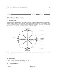
A.6 Phases of the Moon 


Earth has only one natural satellite, the Moon. It is the one of the largest satellites in the solar system. It 

takes the Moon 29.5 days to orbit around the Earth, and it always shows the same side towards the Earth. 

In this activity we are going to study the most noticeable feature of the Moon, the phase. The phase of the 

Moon is a result of the relative angles between the Moon, Earth, and Sun. 

First Quarter 

Full Moon 

12 midnight 

180° 

Earth 

12 noon 

To the Sun 

0° 

New Moon 

Sunlight 

Third Quarter 

Figure A.15: The phase of the Moon seen from the Earth depends on the relative positions of the Sun, 

Earth, and Moon. 

II. Reference 

• 21 st Century Astronomy, Chapter 2, pp. 43 – 46. 


• ball 

• light bulb



Lunar Phases 

1 Turn on the light bulb. We are going to pretend the bulb is the Sun. Hold a ball at arm’s length. 

Which side of the ball is illuminated? Which side is in shadow? 

2 In Fig. A.15, shade the dark sides of the Moon and the Earth. The side facing away from the Sun is 

always in the dark. 

3 We are going to measure all angles from the direction of the Sun (0 ◦ ) in the counterclockwise direction. 

Find the angle to the Moon at each location on the orbit. 

4 Pretend your head is the Earth. The ball is going to represent the Moon. Hold the ball in your hand 

and stretch your arm. As you spin counterclockwise, the Moon orbits around you. Notice that the 

Moon is illuminated by the Sun from different angles with respect to the Earth. At 0 ◦ , your head, the 

ball, and the bulb are aligned in a straight line. You can see only the dark side of the Moon. It is the 

new moon. 

5 Now rotate counterclockwise by 45 ◦ . You should be able to see a crescent moon. Sketch the phase and 

label the phase. Keep rotating by 45 ◦ , and for each angle, sketch and label the phase. 

New Moon 

0° 

Full Moon 

45° 90° 135° 

180° 

225° 270° 315° 

Figure A.16: Lunar phases and corresponding angles between the Sun and Moon. 

What time does a full moon rise? 

We can use Fig. A.15 to find what time the Moon of a particular phase rises or sets. Also, we can find the 

time of the transit. The transit is the time when the Moon, or any celestial body, is exactly on the local 

celestial meridian (LCM). 

1 The local time is defined by the position of the Sun in the sky. When the Sun is on the LCM, it is the 

local noon. From Fig. A.15, find the local time for the transit for each lunar phase.


Table A.15: The transit depends on the phase of the Moon. 

lunar phase rise transit set 

new moon 

first quarter 

12:00 noon 

full moon 

12:00 midnight 

third quarter 

2 The Moon rises 6 hours before the transit and sets 6 hours after the transit. Find when each lunar 

phase rises and sets. 

V. Questions 

1. What is the phase of the Moon if the angle between the Sun and Moon is 150 ◦ in the counterclockwise 

direction? 

2. What is the phase of the Moon during a solar eclipse? 

3. Your younger brother swears that he saw a crescent moon at midnight. Can you trust him? Explain 

your reasoning. 

VI. Credit 





of error in your measurements and how they could have affected the final result. (No, you cannot just say






A.7 The Shape of the Mercury’s Orbit 


Mercury is the innermost planet of the solar system and, therefore, always remains close to the Sun as seen 

from the Earth. It can be seen only right after sunset or right before sunrise. A simple way to determine 

the orbit of Mercury is to use pairs of angles measured at different locations. 

The angle between the Sun and Mercury as seen from the Earth is called the elongation. When the 

elongation reaches its maximal value as shown in Fig. A.17, the line of sight from the Earth to Mercury is 

tangent to Mercury’s orbit. 

Earth's Orbit 

Mercury's Orbit 

Sun 

90° 

Mercury 

θ 

Earth 

Figure A.17: The greatest elongation for Mercury. 

If the orbits of Mercury and Earth were both circular, the greatest elongation would be the same for 

every observation. however, the greatest elongation varies from revolution to revolution because of the elliptic 

shapes of both orbits. In this activity you are going to construct the orbit of Mercury. 

II. Reference 




• compass 

• ruler 

• graph paper



1 Draw a circle of 10 cm radius on a graph paper. This is going to be the Earth’s orbit. Locate the Sun 

at the center of the circle. 

2 Draw a reference line from the center of the circle to the right and label 0 ◦ . This line points to the 

vernal equinox. Earth crosses this line on September 23. 

3 Locate the Earth’s position on your plot of the Earth’s orbit for the date of each entry in Table A.16 

with a protractor. All angles are measured from the vernal equinox in the counterclockwise direction. 

Label each position. 

Table A.16: Greatest elongations of Mercury. 

Date Greatest 

Elongation 

Position of 

Earth 

Feb 14, 2000 18 ◦ E 147 ◦ 

Mar 28 28 ◦ W 187 ◦ 

Jun 9 24 ◦ E 257 ◦ 

Jul 27 20 ◦ W 307 ◦ 

Oct 6 26 ◦ E 12 ◦ 

Nov 15 19 ◦ W 51 ◦ 

Jan 28, 2001 18 ◦ E 131 ◦ 

Mar 11 27 ◦ W 171 ◦ 

May 22 22 ◦ E 239 ◦ 

Jul 9 21 ◦ W 288 ◦ 

Sep 18 27 ◦ E 356 ◦ 

Oct 29 19 ◦ W 33 ◦ 

4 Draw radial lines from the Sun to each of the Earth’s positions you have located. 

5 Use the data in Table A.16 to draw lines of sight from each location of the Earth. Note from Fig. 

A.17 that an eastern elongation (E) is to the left of the Sun as viewed from the Earth. For western 

elongations (W), Mercury is to the right of the Sun. 

6 We know that Mercury is somewhere along the line of sight, but where? On a date of greatest 

elongation, the line of sight is tangent to the orbit of Mercury. That means, Mercury is at the point 

along the line of sight that is closest to the Sun. Locate the position of Mercury for each line of sight. 

7 Now you can find Mercury’s orbit by drawing a smooth curve through, or close to, these positions. 

Remember that the orbit must touch each line of sight without crossing any of them. 

V. Questions 

Draw the major axis for Mercury’s orbit by first finding the points of perihelion and aphelion. These are 

the points on the orbit that are closest to and furthest from the Sun, respectively. They should be at the 

opposite sides of the Sun from each other. 

1. The length of the semi-major axis is equal to a half of the distance between the perihelion and aphelion. 

What is the length of the semi-major axis of Mercury’s orbit in AU?


2. The eccentricity e of an orbit is defined as e = c/a, where c is the distance of the Sun from the center 

of the ellipse and a is the length of the semi-major axis. What is the eccentricity of Mercury’s orbit? 

Calculate the percent error of your measurement from the accepted value of 0.206. 

VI. Credit 











A.8 The Orbit of Mars 


Have you noticed that NASA launches planetary probes to Mars every two years? This is because about 

every two years the Earth and Mars get relatively close to each other and it requires less fuel to send the 

probes to Mars. In this activity you are going to determine the orbit of Mars using the method developed 

by Kepler. 

II. Reference 



• large graph paper 


• ruler 


Mars’ orbital period (687 days) is close to twice that of the Earth (365 days × 2 = 730 days). Thus, every 

time Mars comes back to the same point in its orbit, the Earth has not completed two orbits yet. So if you 

are on the Earth and make an observation of Mars every time Mars is at the same point on its orbit, you will 

see the planet in a different direction with respect to the background stars. The two lines of sight intersect 

at a point on the orbital path of Mars as shown in Fig. A.18. 

The observational data you will use (found in Table A.17) shows Mars’ position on various dates between 

1991 and 1998. Each pair of observations (e.g., A and A’) are made when Mars is exactly at the same point 

in its orbit. The angle to Mars is measured from the vernal equinox as seen from the Earth. The Earth’s 

position is the angle measured from the vernal equinox to the Earth as seen from the Sun. 

All angles are measured from the direction of the vernal equinox in the counterclockwise direction. 

1 Draw a 10-cm radius circle on a large sheet of graph paper to represent the Earth’s orbit and assume 

that the Sun is located at the center of the circle. 

2 Draw a line from the Sun to the right and parallel to the grid lines on the graph paper (see Fig. A.19). 

This line represents 0 ◦ and points toward the vernal equinox. This direction will serve as the reference 

for measuring angles on the Earth’s orbit. The Earth crosses the 0 ◦ line on the autumnal equinox 

(around September 23) and the 180 ◦ line on the vernal equinox (around March 21). 

3 Locate the Earth’s position on your plot of the Earth’s orbit for the date of each observation. Label 

each position. 

4 To determine the angle to Mars on any given date, draw a line from the Earth’s position parallel to 

the 0 ◦ line. This line should be parallel to the grid lines on the graph paper. Use a protractor to 

measure the angle to Mars in the counterclockwise direction from the 0 ◦ line. Two lines for each pair 

of observations will intersect at a point on Mars’ orbit.


Mars' orbit 

★ 

★ 

Background 

stars 

★ 

★ 

Earth's orbit 

A 

θ 

0° 

★ 

A' 

θ' 

0° 

Sun 

Figure A.18: Locating Mar’s position on the orbit. 

5 When you have finished plotting all ten points, use a compass, and by trial and error, draw the best 

circle that fits the plotted points. 

V. Questions 

1. What is the length of the semi-major axis of Mars’ orbit in AU’s? 

2. What is the eccentricity of Mars’ orbit? The eccentricity e of an orbit is defined as e = c/a where c is 

the distance between the Sun and the center of the elliptical orbit and a is the semi-major axis. How 

well does your value agree with the accepted value of 0.093 (i.e., find the percent error). 

3. What is the closest distance of approach for the Earth and Mars in AU?


Table A.17: Observed positions on Mars from the Earth. 

Pairs Date Earth’s 

position 

Angle to 

Mars 

Pairs Date Earth’s 

position 

Angle to 

Mars 

A Mar 21, 91 180 ◦ 83 ◦ G Feb 27, 92 160 ◦ 309 ◦ 

A’ Nov 9, 96 45 ◦ 153 ◦ G’ Oct 19, 97 24 ◦ 254 ◦ 

B May 17, 91 234 ◦ 117 ◦ H Apr 24, 92 213 ◦ 353 ◦ 

B’ Jan 5, 97 107 ◦ 182 ◦ H’ Dec 15, 97 83 ◦ 300 ◦ 

C Jul 13, 91 292 ◦ 150 ◦ I Jun 20, 92 270 ◦ 35 ◦ 

C’ Mar 4, 97 165 ◦ 183 ◦ I’ Feb 10, 98 144 ◦ 345 ◦ 

D Sep 8, 91 347 ◦ 185 ◦ J Aug 17, 92 327 ◦ 73 ◦ 

D’ Apr 30, 97 218 ◦ 169 ◦ J’ Apr 8, 98 198 ◦ 26 ◦ 

E Nov 4, 91 40 ◦ 221 ◦ K Oct 13, 92 19 ◦ 104 ◦ 

E’ Jun 26, 97 276 ◦ 183 ◦ K’ Jun 5, 98 253 ◦ 67 ◦ 

F Jan 1, 92 101 ◦ 265 ◦ L Dec 9, 92 77 ◦ 119 ◦ 

F’ Aug 22, 97 332 ◦ 217 ◦ L’ Aug 1, 98 312 ◦ 109 ◦ 

Mars 

Earth 

Oct 13, 92 

180° 

19° 

Mar 21, 91 

Sun 

104° 

0° 

Dir. of 

Vernal 

Equinox 

Figure A.19: Earth’s orbit. 

VI. Credit 











A.9 Obtaining Ages for Martian Surfaces via Cratering 


As discussed in class, astronomers use crater counts to estimate the relative age of craters. To get the 

absolute age, either the exact cratering rates for ranges of sizes of objects must be known and/or radiometric 

dating must be used to calibrate the number of craters of each size to a particular age. It is typical rather 

than to just “count craters” that astronomers will look at crater densities, ie. the number of craters per 

million square kilometers. In this problem, you will derive ages of 2 different portions of Mars’ surface by 

looking at crater densities. You can fill in all of your numerical answers in the worksheet provided in this 

handout. 

II. Reference 

• 21 st Century Astronomy, Chapter 4, p. 121-2, Chapter 12, p. 308 


• ruler 


IV. Experiments 

Counting craters 

1. In Figure A.21 shown below is near the landing spot of Viking I on the Western Chryse plain. At this 

latitude on Mars, 1 ◦ is equal to approximately 57 kilometers. Use the shown latitudes and longitudes 

to estimate the area of this portion of the surface. You may assume that the same conversion is true 

for longitude as well (it’s not quite right, but close enough for this process). As you can see, the more 

northerly latitude does not quite span the whole width since we’re projecting a sphere onto a flat map. 

2. Repeat the above process for Figure A.22. 

3. In Figure A.21, you’ll be counting the number of craters of a size between 4 and 10 kilometers. The 

easiest way to do this is: 

• Determine what the scaled size is for 4 and 10 km, then use a corner of a piece of paper. Measure 

from the edge, and then fill in a box that contains the acceptable ranges as shown in Figure A.20 

below. 

• Now use your sheet of paper, moving it around to count all the craters that fit in your acceptable 

range. 

4. In Figure A.22, you’ll be counting the number of craters that fall between sizes of 22.6 to 45.3 kilometers. 

Repeat the process you did for Figure A.21. 

5. The above counts are not for 1 million square kilometers, so you will need to correct your counts for 

this. Adjust your counts for both regions as needed to get a number of craters per 1 million square 

kilometers.


cm 

1 

Figure A.20: The shaded area on the paper below the ruler represents the acceptable ranges. This does not 

show the actual values, but just an example. 

6. To get the age, use the graphs showing cratering rate for the different sizes. For Figure A.21, use the 

graph shown in Figure A.23. For Figure A.22, use the graph shown in Figure A.24.


V. Questions 

1. Total area shown in Figure A.21 

2. Total area shown in Figure A.22 

3. Number of craters that fall between sizes of 4 and 10 kilometers in Figure A.21. 

4. Number of craters that fall between sizes of 22.6 and 45.3 kilometers in Figure A.22. 

5. Corrected counts for an area of 1 million square kilometers for: 

(a) Figure A.21 

(b) Figure A.22 

6. Determined age from crater density for: 

(a) Figure A.21 

(b) Figure A.22


Figure A.21: Martian surface near Viking I landing site at 20 ◦ N and 50 ◦ W. Scale is roughly 57 kilometers/degree.


Figure A.22: Martian surface in the Western Chryse Plain at 15 ◦ S and 14 ◦ W. Scale is roughly 57 kilometers/degree.


Figure A.23: Cratering rates for 4 - 10 km craters. Graph taken from website: 

http://www.astro.lsa.umich.edu/users/cowley/Craters/


Crater Density vs. Age 

for Martian surface with craters between 22.6 and 45.3 kilometer diameter 

60 

Crater density (#/1 million sq. km.) 

50 

40 

30 

20 

10 

0 

4 

3.5 

3 

2.5 

Age (billions of years) 

2 

1.5 

1 

Figure A.24: Cratering rates for 22.6 - 45.3 kilometers. Data taken from website: 

http://www.astro.lsa.umich.edu/users/cowley/Craters/




A.10 Optics and Spectroscopy 


Until the introduction of the telescope to astronomy, all observations had been done with the naked eye. 

This limited the resolution and magnification with which we could resolve details on objects even as near 

as the Moon. In addition, the number and type of objects which could be observed was also limited due to 

the relatively small amount of light the human eye can detect. Those objects with an apparent magnitude 

of 6 or greater could not be seen. While spotting scopes had been used by militaries, Galileo was the 

first person to construct a telescope and use it for astronomical purposes and he immediately made many 

important discoveries. Probably the most famous of these early observations was his discovery of four moons 

of Jupiter, now known as the Galilean moons. Galileo observed Io, Europa, Callisto, and Ganymede and 

noticed that they orbited Jupiter, not the Earth. This was one of the final pieces of evidence which caused 

the downfall of the geocentric theory of the solar system. Today even with the ability to look at almost 

any wavelength in the spectrum of light, optical telescopes (those which look at the visible portion of the 

spectrum) are still one of the most fundamental and useful tools for the professional astronomer and the 

only reasonably affordable tool for amateurs. 

Light comes in a wide variety of frequencies (or equivalently wavelengths) from x-rays to radio waves. 

The visible spectrum is but a small portion of the total information available to astronomers. However one 

can still gain a great deal of information by breaking a beam of light into its component pieces by frequency 

(or wavelength). You have probably seen this process using a prism which takes white light from the Sun or 

a light bulb and spreads it out into a range of colors from red to violet. Astronomers use the brightness at 

each of these wavelengths to determine a great deal about the object they are observing. One of the most 

important pieces of information they can obtain by looking at the spectrum is the composition of the object. 

This process is known as spectroscopy. 

In this lab you will learn some of the basic optical rules for constructing telescopes and how astronomers 

use spectroscopy to determine the composition of the object they are observing. 

II. Reference 

• The Cosmic Perspective, Chapter 6, pp 158 – 164, and Chapter 7, pp 172 – 183 


• light box 

• 200 W bulb 

• mirror 

• diffraction grating 

• convex lens 

• concave lens 

• 3 x 5 index card 


• sheet of glass 

IV. Safety and Disposal 

Do not look directly at the Sun or any other bright light source.


V. Experiments 

Optical telescopes 

Optical telescopes come in two varieties, either reflecting or refracting. Reflecting telescopes use a mirror 

to focus the incoming light from the sky to an eyepiece or camera for observation. They are the most 

commonly used type of telescope today as they are easier to construct for large or very large telescopes and 

are cheaper than producing a refracting telescope of the same size. A refracting telescope uses lenses to focus 

the incoming light to the eyepiece or camera. While refractors have their advantages, making very accurate 

and non-distorting lenses of even moderate size is a fairly expensive undertaking. With a mirror you have 

only one surface to make precisely whereas with a lens you must insure that both surfaces of the lens are 

precise and that the lens is clear and uniform throughout the body of the lens. 

Today you will investigate the basic principles behind the assembly of a reflecting telescope including 

determining how light reflects from the surface of the mirror and what happens to the orientation of an 

object seen in a mirror and how that changes with the number of reflections. You will also determine what 

happens to the orientation of an image as seen through various types of lenses. 

(1) Obtain a light box, 200 W bulb and a flat mirror. 

(2) Place one of the black sheets with slits over the appropriate window on the side of the box. Insure that 

the slit is narrow for greater ease of measurement. 

(3) In the area below, place the mirror vertically along the indicated line. 

(4) Using the light box, direct a beam of light so that it strikes the mirror at an angle at the intersection of 

the plane of the mirror and the dotted perpendicular line. Carefully sketch the direction of the incoming 

and the reflected beam of light and label each respectively. You may find it easiest to use the center of 

the beam of light to sketch the beams. 

Mirror 

Figure A.25: Reflection of a beam of light by a mirror. 

(5) Using a protractor, carefully measure the angle of the light beam from the perpendicular line, commonly 

referred to as the normal, for both the incoming and reflected beams and record these angles in Table 

A.18 below. 

(6) Repeat the previous two steps after moving the light box so that the incoming beam approaches the 

mirror at a different angle and again record the measurements in Table A.18 below.


Table A.18: Angles of incidence and angles of reflection. 

Trial Incoming 

Angle ( ◦ ) 

Reflected 

Angle ( ◦ ) 

Trial # 1 

Trial # 2 

(7) From your data, what can you infer about the relationship between the incoming angle and the reflected 

angle of the beam of light? 

(8) Now place the mirror in the space below on the upper horizontal line with the reflecting surface facing 

you. Looking solely in the mirror, attempt to write your name on the line below the mirror. 

Mirror 

(9) Draw and label 4 arrows (one each pointing up, down, left, and right) in the space below. Now place 

the mirror below in the same orientation as before. Compare the directions of the arrows as seen in the 

mirror to those on the piece of paper. 

Mirror 

(10) Using the information from above, what can you say about the orientation of direction as seen with the 

naked eye as that compared to the orientation as seen from a single reflection from a mirror. What do 

you think would happen if you had 2 reflections? Three?


Lenses 

(1) Obtain a 3 × 5 index card, a convex lens, and a concave lens. On the card draw a large arrow. 

(2) Have your partner hold the arrow vertically while you hold the convex lens in the line of sight between 

your eye and the arrow. Move the lens back and forth until the arrow is focused. What is its orientation? 

(3) Have your partner rotate the arrow to point horizontally and again observe the orientation of the arrow 

through the convex lens. What is the orientation of the arrow now? 

(4) Repeat the above two steps for the concave lens noting the orientation of the arrow in both positions. 

(5) Using the information from above, summarize what the concave and convex lenses do to the images 

(orientation and size). 

Spectral lines 

Spectroscopy is one of the most important tools astronomers have in the study of the heavens. By understanding 

the spectrum taken from an object, astronomers can understand that object’s composition, 

rotation, and temperature. 

Spectral lines appear primarily due to transitions of electrons between orbitals in atoms. The differences 

in energy between the energy levels of the electron cause the appearance of lines at different wavelengths (or 

energies). In this portion of the lab you will observe a number of known spectra and then use those spectra 

to identify an unknown spectrum. 

(1) Obtain a diffraction grating for each group member. Observe the five different known spectra. Sketch 

those spectra in the boxes in Fig. A.26. Be sure to label the colors of each line. 

(2) Have your instructor insert the unknown gas into the transformer and observe it with your diffraction 

grating. Sketch the unknown spectrum in the box in Fig. A.27, again labeling each line’s color. 

(3) Compare your unknown spectrum with the known spectra and identify the composition of the unknown.


Element: 

Violet 

Blue 

Green 

Yellow 

Orange 

Red 

400 nm 450 nm 500 nm 550 nm 600 nm 650 nm 

Element: 

Violet 

Blue 

Green 

Yellow 

Orange 

Red 

400 nm 450 nm 500 nm 550 nm 600 nm 650 nm 

Element: 

Violet 

Blue 

Green 

Yellow 

Orange 

Red 

400 nm 450 nm 500 nm 550 nm 600 nm 650 nm 

Element: 

Violet 

Blue 

Green 

Yellow 

Orange 

Red 

400 nm 450 nm 500 nm 550 nm 600 nm 650 nm 

Element: 

Violet 

Blue 

Green 

Yellow 

Orange 

Red 

400 nm 450 nm 500 nm 550 nm 600 nm 650 nm 

Figure A.26: Spectra of known elements.


Element: 

Violet 

Blue 

Green 

Yellow 

Orange 

Red 

400 nm 450 nm 500 nm 550 nm 600 nm 650 nm 

Figure A.27: Unknown spectrum. 

VI. Questions 

1. Explain briefly how an astronomer can determine if the object being observed is moving along the line 

of sight by simply looking at the spectrum from the source. 

2. A common type of telescope is known as a Cassegrain telescope. This is a reflecting telescope and 

consists of a primary mirror which collects the incoming light from the object and bounces it to a 

secondary mirror. The light from the secondary mirror reflects again off a mirror located in a corner 

reflector, and then through a simple eyepiece consisting of a single convex lens. While looking at an 

object through this telescope, how would the image seen through the eyepiece compare with that seen 

by the naked eye? Check your answer by looking through the telescope down the hall towards a lab 

partner.

Chapter B 

Computer Laboratories (CLEA) 

61

62 CHAPTER B. COMPUTER LABORATORIES (CLEA)

CHAPTER B. COMPUTER LABORATORIES (CLEA) 63 


B.1 Astrometry of Asteroids 


Astrometry is one of the fundamental tools of astronomers. Astrometry is the technique of precisely measuring 

the positions of stars and other objects in the sky. By doing so, astronomers can make charts of objects 

in the sky, assigning them coordinates (right ascension and declination). 

Astrometry is useful in that it also helps us to measure parallax (Lab A.1) that occurs over the period 

of a year due to the orbit of the Earth around the Sun. By using those same techniques used in that lab, 

astronomers can measure the distances to nearby stars. In addition we can measure the proper motion of 

nearby objects. Proper motion is the drifting of a celestial object against the background sky 

due to the actual motion of the object itself. 

By using computers and images obtained via CCD cameras, astronomers can determine the coordinates 

of an object to high precision. Even the relatively simple program used in this lab can pinpoint objects to 

within less than 0.1 arcseconds (the size of a dime viewed at a distance of 20 km). 

In recent years, astronomers and the general public have shown increased interest in mapping the orbits 

of asteroids. The reason is to find all near-Earth objects which could conceivably collide with the Earth, 

causing untold damage to society as we know it. To map the orbit of asteroids (or comets), astronomers 

require precise observation of the object’s location over an extended period of time. 

To accurately measure the position of an asteroid, or another object such as a planet, which has no fixed 

position in the sky we need to measure its position relative to other objects whose positions are known. For 

example, look at the image below. It shows two stars whose positions are known, A and B, and a third 

object whose position is not known. Imagine that star A is known to lie at 13 h 0 m 0 s right ascension and 

32 ◦ 0’ 0” declination while B lies at 14 h 0 m 0 s right ascension and 29 ◦ 0’ 0” declination. 

A 

12 

X 

B 

8 

10 18 

Figure B.1: Determining the coordinates of object X

64 CHAPTER B. COMPUTER LABORATORIES (CLEA) 

In this case the unknown object’s coordinates are easy to determine since object X is at the midpoint of 

the line connecting stars A and B. Look at the table below. 

Table B.1: Coordinate data for stars A and B and the unknown object X. 

Object Right 

Ascension 

Declination X Position on 

Image 

Y Position on 

Image 

Star A 13 h 0 m 0 s 32 ◦ 0’ 0” 10 12 

Star B 14 h 0 m 0 s 29 ◦ 0’ 0” 18 8 

Object X ? ? 14 10 

It will have coordinates that are then the values at the midpoint, 13 h 30 m 0 s right ascension and 30 ◦ 30’ 

0” declination. In general of course, things will not be this simple! In addition to the ideal situation above 

being unlikely, the equatorial coordinate system is composed of curves of right ascension and declination, 

not straight lines. Still, a simple coordinate conversion can be done to find the coordinates of the unknown 

object. 

The positions of the known objects will be obtained using a guide catalog, in this case the Hubble Guide 

Star Catalog. This catalog is a compilation of the positions of about 20 million stars (almost all the stars 

greater than 16th magnitude). The program will allow you to identify stars in this catalog and then do the 

coordinate transformation from the object’s coordinates in the image to the equatorial coordinates in the 

sky. 

In this lab you will make simulated observations of the sky, identify an asteroid in pairs of CCD images 

and use measurements of the parallax (by comparing images from two different observatories on either side 

of the United States) to calculate the asteroid’s distance. 

II. Reference 

• CLEA Astrometry of Asteroids Lab, 

http://www.gettysburg.edu/academics/physics/clea/CLEAhome.html 

• Astronomy Lab A.1 


• CLEA Astrometry of Asteroids program 


IV. Observations 

The observations you will be making will be simulated using the CLEA program. You will do the following 

things in this observation: 

• learn to display CCD images of the sky using an astronomical display program 

• blink pairs of images and learn to identify objects which have moved from the time of one image to 

the next 

• call up reference star charts from the Hubble Guide Star Catalog (GSC) 

• recognize and match star patterns on the GSC charts against the stars in your image 

• measure the coordinates of unknown objects on your images using the GSC reference stars 

• measure the parallax of an asteroid and use that to find its distance


Finding the asteroid 

1. Log in to the program by entering all the group members’ names into the appropriate places after 

selecting Log In from the File menu. 

2. Load an image. The image will be approximately 4 arcminutes square and will contain 1992BJ, a faint 

Earth-approaching asteroid. Load the image by selecting File → Load → Image1. A directory listing 

will appear. Select 92jb05.fts and click Open to load it. 

3. The image is now loaded, but not displayed. To display it, select Images → Display → Image1. All 

of the objects in the image are stars except for the asteroid. The image is oriented with west to the 

right and north to the top. Sketch the image in the space below. 

North 

West 

Figure B.2: Your sketch of the CCD image. 

4. To find the asteroid, we will need a second image. Load a second image by choosing File → Load → 

Image2. Select 92jb07.fts and click Open to load it. You can display this image by choosing Images 

→ Display → Image2. This image was taken 10 minutes after the first image you loaded. 

5. To see which dot of light is the asteroid, we need to blink the images. It is easier if we align them first. 

To align and then blink the images, select Images → Blink. You will see only one image, Image1. 

At the bottom right, you will be asked to select an alignment star. If possible, try to select two stars 

which lie opposite each other (on a diagonal is best if possible). Choose the first star and note it in 

your sketch labeling it Star 1. Click on Continue and select a second star in the same manner. Again, 

label this star on your sketch labeling it Star 2. Click on Continue.


6. You will now see Image 2 and be asked to identify Star 1 in the image. Click on Star 1 then Continue 

and repeat for Star 2. You may find that the computer has already figured out these stars for you. 

7. Click on Blink now to blink the stars. You will see the computer flip back and forth now between the 

two images. You should be able to identify the asteroid. Occasionally there are defects in the image 

where a bright spot will appear in one image, but not in others. This is often due to a cosmic ray 

striking the detector. Be careful to insure that you have correctly identified the asteroid. 

8. Once you’ve identified the asteroid you can stop the blinking by clicking on Stop. On your sketch 

carefully label the asteroid’s position in Image 1 as 05 and sketch its new position in Image 2 labeling 

it 07. 

9. Once you have completed this, repeat this procedure by loading images 92jb08, 92jb09, 92jb10, 

92jb12, and 92jb14. Continue to use 92jb05 as Image 1 and loading a new Image 2. 

10. Once you have labeled the positions of the asteroid from each image in your image you should be able 

to draw a line through the path of the asteroid. What direction is it moving? 

Measuring the asteroid’s position 

Now that the asteroid is identified, the next step is to determine the position of the asteroid. As noted 

earlier, the computer will do most of the work in changing from the CCD image’s coordinates to equatorial 

coordinates. To do this, the program needs to know the actual positions of at least three of the stars in your 

image (the more stars you can identify the better in general). You will identify stars by using the Hubble 

Guide Star Catalog (GSC). This catalog was originally created to help point the Hubble Telescope. For each 

of the images you loaded previously, you will determine the coordinates of the asteroid by: 

• telling the GSC the approximate position of the center of the image so that it can draw a map of 

known stars in that vicinity; 

• identify at least three GSC stars that are also on the image as reference stars; 

• point and click on these reference stars so that the computer knows which ones have been chosen ; and 

• point and click on the asteroid so that the computer can calculate its position. 

1. If you still have 92jb05 loaded as Image 1 use that. If not reload it. Once loaded, choose Images → 

Measure → Image1. A window will open asking you to input approximate coordinates of the center 

of your image. Enter the coordinates found in Table B.2 for 92jb05. Set the field size to 8 arcminutes. 

The images are about 4 arcminutes in size, but this will leave you some margin for error in finding 

your reference stars in the image. Remember the scale is different when identifying your stars! Click 

OK. 

2. Now identify at least three stars in the GSC map with the stars in your image. When you see the 

match, identify them by sketching and labeling them from 1 – 3 in the area below. The stars should 

be well separated for the best results. 

3. Now click on the first reference star you chose in the GSC map window. Data on the star’s position 

from the GSC will appear. Record the data in Table B.3 below. 

4. Once you have selected your reference stars, choose Select Reference Stars from the dialog box at 

the bottom center of your screen. Click OK. If you’ve only selected three stars, the computer will 

warn you that more stars will produce more accurate results. If you can only find three, then click 

NO to continue.


North 

West 

Figure B.3: Your sketch of the reference stars. 

5. You will now be asked to point to reference star 1, then star 2 etc. in the Image 1 window (92jb05). 

Click each star in turn making sure it matches the star in the GSC map. Remember the scales are 

different! After you’ve done the first two stars the computer will estimate the positions of the remaining 

stars. If the star is anywhere inside the square box, you can just click OK to accept its choice. 

6. Once all the reference stars have been selected, you will be asked to identify the unknown object. Click 

on the asteroid and a dialog box will appear with the asteroid’s coordinates. Record these results down 

in Table B.4. Hit OK to accept this solution and repeat this process for the remaining images. You 

should also record this data on the computer - just hit Yes when it asks you if you would like to do 

this. Make sure to record the correct image name (92jb**) when asked for the object name.


Table B.2: Information on images - data taken from the National Undergraduate Research Observatory on 

May 23, 1992. 

File Name 

RA (2000) of 

image center 

(h m s) 

DEC (2000) of 

image center 

( ◦ ’ ”) 

TIME (UT) of 

mid-exposure 

(h m s) 

Exposure 

length (s) 

92jb05 15 30 44.30 11 15 10.4 04 53 00 30 

92jb07 15 30 44.30 11 15 10.4 05 03 00 120 

92jb05 15 30 44.30 11 15 10.4 05 09 00 30 

92jb05 15 30 44.30 11 15 10.4 06 37 30 180 

92jb05 15 30 44.30 11 15 10.4 06 49 00 30 

92jb05 15 30 44.30 11 15 10.4 06 57 00 120 

92jb05 15 30 44.30 11 15 10.4 07 16 00 30 

Table B.3: Reference star coordinates 

Reference 

Star 

# 1 

# 2 

# 3 

ID # RA DEC 

7. When you have measured the position of the asteroid in all of the images, print your data using Report 

→ Print. 

Table B.4: Position of asteroid 1992JB 

File Name Time (UT) RA (h m s) DEC ( ◦ ’ ”) 

92jb05 

92jb07 

92jb08 

92jb09 

92jb10 

92jb12 

92jb14 

Measuring the distance to 1992JB 

In this section you will find the distance to the asteroid using the method of parallax similar to what was 

discussed in Lab A.3. You will use two images taken simultaneously at two different observatories on different 

sides of the United States and the resultant parallax to find the distance. The distance to the star can be 

found by: 

( ) B 

d = 206, 265 , (B.1) 

θ 

where d is the distance of the asteroid from the Earth, B is the baseline or the distance between the observatories, 

and θ is the measured parallax angle measured in arcseconds. Using the program, the measurement of


the parallax angle is quite quick and accurate. The two telescopes are located 3172 km apart. One telescope 

is located at the National Undergraduate Research Observatory in Flagstaff, AZ and the other is at Colgate 

University in Hamilton, NY. 

1. First you need to load the two images, ASTEAST as Image 1 and ASTWEST as Image 2. Load 

and display these two images as you have done previously. The images will not look exactly the same 

as one is more sensitive and they have different sized CCD chips on on which the images were taken. 

2. Find the asteroid in the images by blinking as you did previously. 

3. Look at image ASTEAST and compare the asteroid’s position in it as compared with its position in 

ASTWEST. Does the asteroid appear to be further east or west in the ASTEAST image? 

4. Is this what you expected? Explain by drawing a diagram in the space below. hint: think about the 

position of the telescopes on the surface of the Earth 

5. Now measure the coordinates of the asteroid in each image as you did previously and record the data 

in Table B.5 below: 

Table B.5: Position of asteroid 1992JB 

File Name RA (h m s) DEC ( ◦ ’ ”) 

ASTEAST 

ASTWEST 

6. You should find that there is a very small difference in both the right ascension and declination for 

the asteroid’s position. To calculate the parallax angle, we need to calculate the difference in the the 

position of the asteroid in the two images in arcseconds. 

7. You should be able to just subtract the declinations as it should differ solely in the arcsecond portion 

of the measurement. 

• ∆DEC(”) = 

8. To calculate the difference in right ascension, first subtract the two right ascensions - this should also 

be simple as they should differ only in the seconds portion of the measurement.


• ∆RA(s) = 

9. We need to convert this measurement in seconds to arcseconds. At the equator, every 15 ◦ of RA 

corresponds to 1 hour of RA (360 ◦ for every 24 hours). However this isn’t true as one moves from 

the celestial equator as the right ascension lines come together at the pole. To correct for this, the 

conversion is: 

∆RA(”) = 15 × ∆RA(s) × cos(DEC), 

(B.2) 

where DEC is the declination of the asteroid from Table B.5 in degrees (it is about 11.25 ◦ ). Convert 

your RA difference into arcseconds. 

• ∆RA(”) = 

10. The total parallax angle is found using the Pythagorean theorem: 

Calculate your parallax angle. 

• θ(”) = 

θ = √ (∆RA) 2 + (∆DEC) 2 

(B.3) 

11. Now calculate the distance of the asteroid using Eq. B.1. Recall the baseline is 3172 km. 

• d = 

V. Questions 

1. How does the distance for the asteroid compare with the distance to the Moon? 

2. We cannot use parallax to measure objects at great distances. What prevents this? 

VI. Credit 

To receive credit on this lab, you must turn in the data from your observations (one print out per group 

is fine), the position data from the parallax measurements along with the parallax angle and distance 

calculations, and the answers to the above questions.



B.2 Rotation of Mercury 


Because Mercury is a relatively small planet with very few large surface features and since it is always near 

the Sun in the sky, it is very difficult to determine the rotation rate of Mercury by direct optical observation. 

In recent years though, astronomers have used radar techniques to measure the rotation rate of both Mercury 

and Venus. 

The basic principle is to send a pulse of radar at Mercury. Depending on its position relative to the 

Earth it will take approximately 10 minutes to a half hour to reach Mercury, reflect off the surface, and 

return to Earth. Because the pulse spreads out as it travels (just as the waves from a pebble dropped into 

a pond spread), the pulse hits the whole surface of the planet. The first point to reflect the pulse is called 

the sub-radar point. See Figure B.4 below. The pulse then continues to travel past the surface of Mercury, 

reflecting back at very small time intervals (microseconds, or millionths of a second) after the sub-radar 

point. As we sample the reflected wave with our detector, we can obtain information about different points 

on the surface of Mercury. 

The rotation rate can be discovered due to the Doppler effect. Recall that the Doppler effect is the 

change in frequency (or wavelength) caused by any relative radial motion between the source and the observer. 

Motion decreasing the distance between the source and the observer results in a shortening (or bluing) of the 

wavelength - this is known as a blue shift because the wavelength is getting shorter and blue is the shortest 

portion of visible light- this is equivalent to an increase in the frequency. Motion increasing the distance 

between the source and observer causes an increase (or reddening) of the wavelength and this is known as a 

red shift - this is equivalent to decreasing the frequency. Since one edge is moving towards us, that edge 

will show a redshift relative to the planet as a whole while the opposite edge shows a blueshift. Again, see 

Figure B.4. 

Reflected pulse has higher frequency than 

the planet as a whole (blueshift) 

Mercury 

v r 

Sub radar 

Reflected pulse shifted solely by the 

planet's orbital velocity 

v r 

point 

Reflected pulse has lower frequency than 

the planet as a whole (redshift) 

v r 

Figure B.4: Doppler shift from various portions of a rotating object.


As noted above there are two motions which will result in Doppler shifts of our radar pulse - the orbital 

velocity of the planet and rotational velocity of the planet. The orbital velocity can be determined by looking 

at the reflection from the sub-radar point. At the sub-radar point, the rotational velocity, v r , will not cause 

a shift because it is perpendicular to the line of sight to this point so any shift seen in the reflected pulse 

from the sub-radar point is due solely to the orbital motion. As additional reflected pulses are examined 

larger areas of the planet are reflecting pulses which are away from the sub-radar point so that there will be 

both a redshift and blueshift in the returned signal. See Figure B.5 for an example. 

Lower frequency 

(redshifted edge) 

Higher frequency 

(blueshifted edge) 

Frequency of reflected pulse 

(difference from original frequency) 

Figure B.5: Example of a reflected radar pulse signal. 

In this lab you will simulate an actual radar observation of Mercury using a computer program. Using 

the program allows us to accurately simulate the radar observations a modern astronomer would make. 

The program will accumulate a series of 5 different pulse returns - the sub-radar reflected signal in 

addition to 4 others spaced shortly after the return of the sub-radar signal. From these signals you will be 

able to calculate the rotational velocity of Mercury and from that calculate its rotational period. Using the 

sub-radar signal you will be able to calculate the orbital velocity of Mercury and from that determine its 

orbital period. 

II. Reference 

• The Cosmic Perspective, p. 167 

• CLEA Radar Measurement of the Rotation of Mercury lab, 

http://www.gettysburg.edu/academics/physics/clea/CLEAhome.html 


• CLEA Radar Measurement of the Rotation of 

Mercury program 



The observations you are making will be simulated using the CLEA program. You will do the following 

things in this observation: 

• calculate the position of Mercury and point a radio telescope at it 

• send a radar pulse at Mercury


• calculate various geometrical patterns necessary to interpret the data 

• measure the shift in frequency of a radar pulse reflected off of Mercury and from that calculate Mercury’s 

rotational velocity and period 

• measure the shift in frequency of a radar pulse reflected off of Mercury from the sub-radar point and 

from that calculate the orbital velocity and period of Mercury. 

Taking Data 



2. Select Start. Press the Tracking button so that the telescope will track Mercury. 

3. Select Ephemeris from the main menu; this will start a process to calculate the position of Mercury. 

Enter your group’s time and date into the appropriate boxes, then press OK to compute the position of 

Mercury. Leave the window with the computed position on the screen and select the Set Coordinates 

button. 

4. Once you okay the coordinates to the telescope, it will begin to slew (move rapidly) to those coordinates. 

Once slewing is complete, you may send a pulse by hitting Send Pulse. A graphical representation 

will then appear showing the progress of the pulse. The orbital size scale is correct and the pulse will 

travel at the speed of light relative to the scale of the image on the screen. The planet and Sun sizes 

are however greatly exaggerated in this view. 

5. The return pulse will be spread out over several hundred microseconds due to the curved surface of 

the planet. You will obtain data for 5 different times. The first will be the sub-radar point reflection 

followed by one at 120 microseconds and then 3 more at 90 microsecond intervals after this (210, 300, 

and 390 microseconds after the sub-radar pulse is received respectively). 

6. It will take at least 10 minutes (up to 30) for your pulse to arrive at Mercury, be reflected, and return 

to your telescope. While this is occurring, move on to the next section and begin your calculations. 

7. A series of 5 windows shown for each of the times will appear on the screen. You will need to measure 

the spread by recording the left-most and right-most shoulders of the pulse. To measure the values of 

the frequency, you need only position the cross-hair in the window and click the left mouse button. 

The value of the difference in frequency will appear in the window. You should position the cross-hair 

so that it is at the edge of the shoulder of the pulse, where the pulse begins to fall towards zero. Record 

your data for the left and right frequency values in Table B.6 for all of the data except the data from 

the reflection due to the sub-radar point. 

8. Finally, measure the central peak of the sub-radar point and record that information in Table B.6. 

Note that this is just the shift from the original frequency. 

Calculations 

1. You will need to know some geometric quantities to determine the rotation rate. Since you are observing 

signals that are reflecting from different portions of the surface. Recall that the a Doppler shift occurs 

only when there is relative motion between the source and the observer along the line of sight. As seen 

below in Figure B.6, the Doppler velocity you measure is only a fraction of the total rotational velocity 

of Mercury. You can find the total velocity by using similar triangles. Note that the triangle which 

contains x, y, and R is similar to that which contains v o and v r . Here d is the extra distance along the 

line of sight that the radar wave travels, x is the difference between the radius of Mercury, R, and d, v o 

is the velocity responsible for the measured Doppler shift, and v r is the rotational velocity of Mercury.


Mercury 

d 

x 

y 

R 

c∆t 

v o 

v r 

Figure B.6: Geometrical quantities for calculating Mercury’s rotation velocity 

2. We can calculate the distance d because we know the rate at which the radar wave is traveling, 

c = 3.0 × 10 8 m/s, and the time it is traveling extra as compared to the wave reflected from the subradar 

point. The time delay is almost equal to the times that we measure the reflected waves back at 

Earth. However, those times are the total delays and the wave has to travel actually twice the distance 

d, once ingoing and once upon reflection. We just need to divide the distance we get using our delayed 

observation times by two, so 

Recall a microsecond is 10 −6 seconds. 

d = 1 2 c∆t. 

3. The distance x is just the difference between the radius of Mercury and the distance d. The radius of 

Mercury is 2.42 × 10 6 meters. 

x = R − d 

(B.5) 

4. To calculate y, we just use the Pythagorean theorem: 

(B.4) 

y = √ R 2 − x 2 

(B.6) 

After you have calculate these quantities for the 4 different time delayed signals (120, 210, 300, and 

390 microseconds), return to the program and measure the frequency shifts. Once those are measured 

and your data recorded, come back here to the next step in the calculations. 

5. Calculate the total frequency shift due to the rotational velocity alone. Note that the total shift you 

measure is twice as big as the real shift because one side is rotating towards you while the other is 

rotating away from you. The total shift then is: 

∆f total = 1 2 (∆f right − ∆f left ) 

(B.7) 

Record this for each of the delayed signals in Table B.6. 

6. Calculate the corrected frequency shift ∆f c because this is a reflected pulse. The total frequency shift 

calculated above is still two times too big because the wave will initially look shifted to the surface of 

Mercury as it approaches and shifted from that in the reflected pulse as seen from Earth so: 

∆f c = ∆f total 

2 


(B.8)


7. Calculate the velocity from the Doppler shift, v o . Note that f is the frequency of the initial pulse 

which is displayed at the lower left corner of the main window. To match units make sure that you 

use f in Hz, not MHz (10 6 Hz). 

( ) ∆fc 

v o = c 

(B.9) 

f 


8. Finally, calculate the rotational velocity, v r . This can be done using similar triangles: 

v r 

= R v o y , (B.10) 

( ) R 

v r = v o . (B.11) 

y 

9. You can now calculate the rotational period of Mercury. We know the distance Mercury rotates through 

and its speed so we can calculate the time: 

P rot = circumference 

v r 

= 2πR 

v r 

(B.12) 

(B.13) 

You can convert this time from seconds into days by dividing by the number of seconds per day, 86,400. 

10. Calculate an average value for the period of rotation for Mercury. How does this compare to the 

accepted value of 59 days? Calculate the percent error in your measurement. 

You will now calculate the orbital velocity of Mercury using the information from the sub-radar point. 

1. Using the reflected pulse from the sub-radar point, you can calculate the orbital velocity of Mercury. 

The shift you recorded is just twice the total shift because it is an echo. You can use Eq. B.8 – B.9 

making only one change - in Eq. B.9, v o will be the orbital velocity. Calculate Mercury’s orbital velocity. 

Write your number for the orbital velocity on the board and next to it a sketch of the orientation of 

the Sun, Earth, and Mercury for your chosen observation date (you will reference this data later). Do 

not quit the program!


Table B.6: Mercury Data Table 

∆t (µs) 120 210 300 390 

d (m) 

x (m) 

y (m) 

f left (Hz) 

f right (Hz) 

∆f total (Hz) 

∆f c (Hz) 

v o (m/s) 

v r (m/s) 

P rot (days) 

V. Questions 

1. The ephemeris data you recorded initially gave you the distance to Mercury in terms of the astronomical 

unit. How big is an astronomical unit in km? You can use your data to find out. Do a unit conversion 

using your round-trip light travel time to calculate the number of kilometers in 1 AU. The first term 

is written below along with the units you should end up with. 

( # km 

1 AU 

) [ 

= 

time 

distance (AU) 

] 

× (B.14)


2. Look at the blackboard showing the lab results for the orbital velocity and their associated sketches. 

Can you explain the results? In particular, why would it be difficult for you, the astronomer, to obtain 

an accurate measurement of the orbital velocity of a planet (not just Mercury) using Doppler shift? 

VI. Credit 

To receive credit for this lab you must turn in the data from Table B.6, your calculated values for orbital 

and rotational velocity and the rotational period, and the answers to the above questions.

78 CHAPTER B. COMPUTER LABORATORIES (CLEA)



B.3 Jupiter’s Moons 


Galileo Galilei was the first to record seeing moons surrounding Jupiter. The four moons he observed are 

now known as the Galilean moons. They are, in order of increasing orbital distance, Io, Europa, Ganymede, 

and Callisto. Although the moons follow elliptic orbits, they appear to move in a linear, rather than circular 

fashion about Jupiter. This is due to the fact that the plane of the moons’ orbits lies nearly in the ecliptic 

plane. Recall that the ecliptic plane is the plane which is described by the path which the Sun follows through 

the sky and that most of the planets’ orbits lie within or very near this plane. 

Because of this projected view of circular motion onto a line, the observed distance from Jupiter when 

plotted should appear as a sine curve. The period of this sine curve is period of the Moon’s orbit. By 

measuring the period of the orbit and the semi-major axis from a graph, you can use Kepler’s third law 

P 2 = 

a 3 

M Jupiter 

(B.15) 

to calculate the mass of Jupiter. 

In this lab you will simulate an actual set of observations on the Galilean moons using a computer 

program rather than making actual observations. Using the program allows us to accurately simulate making 

observations that a modern astronomer would make using a CCD camera to obtain images through a 

telescope. 

The program will allow you to make a series of observations. On some “nights” it will be cloudy and you 

will not be able to obtain any data for that night. Using your data set you will be able to find the orbital 

periods for each of the Galilean moons and then be able to calculate Jupiter’s mass using Kepler’s third law. 

II. Reference 

• 21 st Century Astronomy, Chapter 3, pp. 76 – 77, 81 – 82 (Kepler’s 3 rd law). 

• CLEA Jupiter’s Moons lab manual 


• CLEA Jupiter’s Moons program 



The observations you will be making will be simulated observations using the CLEA program. You will do 

the following things in this observation: 

• measure the apparent positions of the Galilean moons relative to Jupiter for a number of days (different 

lab groups will be given different periods of time over which to make the observations) 

• plot the apparent positions of each moon versus time on graph paper, and draw a best fit sine curve 

through the data


• use your graphs to determine the semimajor axis and period of each moon 

• use the values from your graphs to determine an average mass for Jupiter 

Observation 

1. Start the Jupiter program by double-clicking on the Clea jup icon. 



3. Select Run from the File menu. Enter the start date and time given to your group by the instructor. 

You can use the default observation interval or you can set it by selecting File → Preferences → 

Timing and changing it to your preferred value. Setting it to a shorter time interval may be useful. 

4. The observation field can be displayed at different levels of magnification. You can change it by clicking 

on the 100X, 200X, 300X, and 400X buttons at the bottom of the screen. To improve the accuracy 

of your measurement, you should use the largest possible magnification which allows you to make your 

measurement. 

5. In order to measure the observed distance of the moons from Jupiter, move the mouse pointer until 

the tip is centered on each moon. Hold down the left mouse button and the cursor will change to 

a cross-hair. Center the moon in the cross-hair and information about the moon will appear in the 

lower right corner of the screen. The information will include the name of the moon, the x and y 

pixel location on the screen, and the perpendicular distance (in units of Jupiter’s diameter) from the 

Earth-Jupiter line of sight as well as an E or W to signify whether it’s east or west of Jupiter. Record 

this information using Record Observations. Be sure to enter a “E” or “W” to signify the position 

of the moon relative to Jupiter. 

6. Once you have recorded the data for each of the moons on that date, continue making observations on 

consecutive observation intervals by clicking on the Next button. You need to observe for at least 18 

observation intervals. 

7. After completing your observations, you should save your data. The data can be saved using File → 

Data → Save. A copy of your data should be turned in with your lab. You can do this by using Data 

→ Print → Data Table. 

8. You now need to analyze your data. This can be done using the program. Select File → Data → 

Analyze. 

9. Choose Select → Moon and select one of the moons to analyze. Start with Ganymede. 

10. Choose Plot → Fit Sine Curve → Set Initial Parameters. You need to set 3 parameters to help 

the program fit the data: t-zero, period, and amplitude (in units of Jupiter diameters). T-zero is the 

time when the sine wave first starts a cycle, the period is the time it takes the moon to orbit Jupiter, 

and the amplitude is the semimajor axis of the orbit. An example graph showing these quantities 

appears in Fig. B.7 below. You will need to estimate values of these quantities from your data. 

11. Adjust the values for the three quantities using the scrollbars to obtain a best fit. Note you may need to 

reset the initial values if they were not close because the scrollbars have a limited range of adjustment. 

Once you have found your best fit, print that page by choosing Plot → Print Current Display. 

12. Repeat the above procedure for the next 3 moons.


Sample Moon Data 

4 

2 

Position (Jupiter diams.) 

0 

−2 

t−zero 

period 

amplitude 

−4 

0 2 4 6 8 

Time (days) 

Figure B.7: Sample graph of data for a moon. 

V. Questions 

1. Please fill in the following table using your data and actual values. 

Moon 

Table B.7: Values of orbital quantities for Jupiter’s moons. 

Measured 

period (days) 

Actual period 

(days) 

Measured 

semimajor axis 

(Jup. diams.) 

Actual 


(Jup. diams.) 

Io 1.769 2.949 

Europa 3.551 4.692 

Ganymede 7.155 7.483 

Callisto 16.689 13.169 

2. Using Eq. B.15, calculate a mass for Jupiter from each moon’s data. Note you will need to convert 

the values in your table above to AU (astronomical units) and years for the semimajor axis and period 

respectively. 

Jupiter’s diameter = 9.53 × 10 −4 AU. 

(B.16) 

Fill in the following table with your data. Also recall that the mass you calculate for Jupiter will be 

given in terms of the mass of the Sun. Once you have calculated the average in terms of the Sun’s 

mass, convert that to kilograms (M ⊙ = 1.99×10 30 kg) and find the percent error in your measurement. 

The actual mass of Jupiter is 1.90 × 10 27 kg.


Table B.8: Value of Jupiter’s mass. 

Moon 

Io 

Measured period 

(years) 

Measured 


(AU) 

Jupiter’s mass 

(Sun’s mass) 

Europa 

Ganymede 

Callisto 

Average mass of Jupiter (M ⊙ ) = 

Average mass of Jupiter (kg) = 

percent error of Jupiter’s mass measurement = 

3. If you did not change the observation interval, you may have had trouble analyzing the data for Io. 

Why? How would you change the time interval to make your analysis simpler? 

VI. Credit 

To receive credit for this lab, you must turn in all of the data from your observations, copies of your graphs 

for each of the moons, the calculated values from Tables B.7 and B.8 as well as your answers to the above 

questions.

Chapter C 

Observations 

83

84 CHAPTER C. OBSERVATIONS

CHAPTER C. OBSERVATIONS 85 

C.1 Constellation Quiz: Get To Know Your Night Sky! 


There are 88 constellations in the sky. From Radford you can see 48 of them. However, due to the revolution 

of the Earth around the Sun, visible constellations depend on the time of the year. For example, fall 

constellations, such as Pegasus, occupy most of the sky in the fall. The celestial sphere and thus constellations 

slowly rotate toward the west by about 1 ◦ a day as the Earth orbits around the Sun. In this activity your 

familiarity with the fall constellations and celestial objects are tested. 

II. Reference 

• Constellation chart posted on class web page: http://peloton.radford.edu/astr111/sky.pdf - this 

will be updated monthly. 

III. Observations 

Become familiar with the following constellations (and celestial objects within them) that you can find in 

the sky in the fall. Fig. C.1 might be useful. If you still have trouble identifying the objects in the sky, ask 

your instructor for help. 

Constellations 

• Andromeda 

• Aquila 

• Bootes 

• Cassiopeia 

• Cygnus 

• Corona Borealis 

• Heracles 

• Lyra 

• Pegasus 

• Perseus 

• Sagittarius 

• Scorpius 

Stars 

• Altair (Aquila) 

• Arcturus (Bootes) 

• Antares (Scorpius) 

• Deneb (Cygnus) 

• Fomalhaut (Piscis Austrinus) 

• Polaris (Ursa Minor) 

• Vega (Lyra) 

Asterisms 

• Big Dipper (Ursa Major) 

• Great Square (Pegasus) 

• Great Summer Triangle (described by Vega, 

Deneb, Altair) 

• Little Dipper (Ursa Minor) 

• Northern Cross (Cygnus) 

Deep Sky Objects 

• M31 Andromeda Galaxy (Andromeda) 

Planets 

• Saturn 

You need to be able to find any fifteen of the above planets, constellations, stars, and celestial objects 

during the observation night (when the sky is clear).

86 CHAPTER C. OBSERVATIONS 

Ursa Major 

North 

Ursa Minor 

Lynx 

Camelopardalis 

Polaris 

Draco 

Gemini Auriga 

Cassiopeia 

Cepheus 

Hercules 

Lyra 

Vega 

Perseus 

Lacerta 

Deneb 

Cygnus 

East 

Orion 

Taurus 

Andromeda 

Triangulum 

Aries 

Pegasus 

Vulpecula Sagitta 

Altair 

Delphinus 

Aquila 

Equuleus 

West 

Pisces 

Eridanus 

SE 

Cetus 

AquariusCapricornus 

SW 

Fornax 

Microscopium 

Piscis Austrinus 

Sculptor 

Phoenix 

South 

Grus 

Figure C.1: Fall sky in Radford at 8:00 pm on October 1.



C.2 The Sun and Its Shadow 


Although one many not think of making astronomical observation in the daytime, there are a number of 

activities that one can undertake in broad daylight. Those include observations of the Sun and Moon. In this 

exercise, we will study the motion of the Sun by looking at the shadow of a vertical pencil and its changing 

rising and setting location. This lab will be worth 3 lab grades (30 points) and will take a maximum of 6 

hours (per person). 

II. Reference 

• 21st Century Astronomy, Chapter 2, pp. 9 – 14. 


• large piece of cardboard 

• large sheet of paper 

• pencil 

• piece of clay 

• marking pen 

• watch or clock 


• magnetic compass 

IV. Safety and Disposal 

Do not directly look at the Sun. 

V. Observations of the Sun’s Shadow 

You will need to make multiple observations of the Sun throughout the day and at different times of the 

semester. These observations must be made at the same location each time. It is recommended that the 

observations for measuring the Sun’s shadow be spaced at least two or three week intervals. The observations 

of the Sun’s rising and setting location must be done from the same location as well, though not necessarily 

the same as that used for measuring the Sun’s shadow. 

Sun’s shadow 

In this portion of your project, you will observe the changing length of the shadow cast by a simple sundial 

over the course of a day. Your group must have a total of four of these measurements over the semester, 

preferably one from each group member. To record the Sun’s shadow, you will create a simple sundial as 

shown below. 

1. Tape the sheet of paper on the cardboard. 

2. Place the cardboard where it will receive sunlight during the majority of the day. 

3. At the middle of the sheet of paper, place an ×.


4. Using a magnetic compass orient the cardboard so that the longer side of the sheet is aligned with the 

East-West line. After leveling the cardboard, draw a straight line from the base of the pencil to due 

North using the compass. This is the magnetic North-South line. 

5. Stand a pencil vertically using a piece of clay centered on the ×. The pointed end of the pencil must 

be pointing up. Once standing, record the height from the paper to the tip of the pencil somewhere 

on the sheet of paper. 

Sun 

N 

E 

Cardboard 

7:05 

10:07 

8:59 

8:02 

S 

W 

Sheet 

Figure C.2: Tracing the Sun’s shadow. 

6. Mark the tip of the shadow of the pencil at approximately hourly intervals during the day. Make more 

frequent observations, if possible, during the middle of the day. Be sure to record the time of each 

observation. 

7. When you are finished, draw a smooth curve going through your observation points on the sheet. 

Determining local noon 

You can use your observation to determine the relationship between local noon and clock time. Local noon 

is the time when the Sun is due south and transiting your local celestial meridian. It is at this time, that 

the Sun reaches its maximum altitude. 

1. What does this say about the length of the shadow of the pencil at the local noon? Note that the 

variation in the length of the shadow near noon is quite small. 

2. How can you determine the shortest shadow? There are several ways of doing this; some are more 

accurate than others. Find the one that you think gives a reasonably accurate answer.


3. How do you account for the difference between the local noon obtained from the shadow and the noon 

of the Eastern Standard Time? 

Finding geographic north 

You can find the direction of geographic North using your observation. , that is, the direction of your local 

line of longitude from using your observation. 

1. Find the point on the curve you drew on the sheet closest to the base of the pencil. Draw a line between 

this point and the × at the center of the sheet. 

2. Measure and record the angle between this line and the magnetic North-South line using a protractor. 

3. Why do the geographic and magnetic North-South lines point in different directions? 

VI. Observations of the Sun’s Rising and Setting Location 

In this portion of your project, you will observe the changing position of the Sun’s rising and setting location. 

All of these observations must take place at the same spot. 

Observations 

1. Choose a location from which all your observations will be made. It must be easily accessible to all 

members of your group. If a single location will not suffice, part of the group can work at one location 

and the remainder at a second. If this is the case, one group should do sunrise and the other sunset. 

2. Take two photographs, one facing due east and the other due west. A digital photograph will probably 

work best. Make sure that the image has a large field of view (ie, don’t zoom). You can use a compass 

to get the directions of due east and west. Mark the location of due east and west on the photographs. 

3. Observe the sunrise and sunset. Your group must make a total of 20 observations of both sunset and 

sunrise (total of 40) spread over a period of 2 months. Mark on the photograph the rise or set location 

relative to landmarks in the photo. Also record, on a separate sheet, the rise or set time.


VII. Write-Up 

Turn in your two photographs, your table of rise and set times, and a minimum of four shadow observations. 

Write a short (2 pages maximum) report summarizing your data. Include in your report a description of why 

the rise and set times and positions change over the year as well as a discussion of why the shadow tracings 

you made differ over time. Finally, make sure that your report answers all of the questions throughout the 

text of the lab. 

VIII. Extra credit 

1. Using your data from each shadow plot, determine mathematically the maximum altitude the Sun 

reached for each observation. You will need to use the length of the pencil and the length of the 

shadow to determine this. Hint - set up a right triangle to find the altitude.



C.3 Moon Observation 


The Moon is, when its up, the most obvious object in the night sky and the second most obvious object seen 

during the day (again, when it’s up). There are many unique features on the Moon which you can see with 

the naked eye such as the maria, the dark lava “seas” and the craters. Through a telescope you can see far 

more detail and get a better view of the mountain ranges, craters and maria. 


• telescope 

• CCD camera (possible) 

III. Observations 

In this lab you will make an observation of the Moon through a telescope. If possible, you will also take an 

image of the Moon using a CCD camera and then process that image. Ideally you will make this observation 

at a time when the Moon is not near the full moon phase. A partially illuminated Moon will give you better 

contrast and hence better surface detail. 

Observation 

1 Point the telescope at the Moon, finding it first in the finder scope, then once it’s centered switching 

to the main telescope. 

2 Focus the image and sketch the view of the Moon in the space provided in an observation sheet. Also 

record all of the information asked for. Be sure to capture as much detail as you can. Drawing a few 

crates is not sufficient as you will need to use your drawing to identify regions on the Moon. 

3 If available, ask your instructor for instructions to use the CCD camera to take an image of the Moon. 

IV. Write-Up 

Using your sketch of the Moon and Redshift (software installed in the Curie computer room (CU 143), 

identify at least 3 features in your sketch. Discuss briefly some characteristics of these features (how they 

were formed, roughly how old they might be etc.). 

V. Credit 

To receive credit in this lab, you need to turn in your observation sheet and write-up. If you obtained an 

image with the CCD camera, you need to email that to your instructor as well.




C.4 Sunspot and Prominence Observation 


Sunspots are areas on the Sun which appear darker. We have known about sunspots for hundreds of years, 

since Galileo first studied them. Sunspots vary in size but are typically about the same diameter as the 

Earth. Sunspots are related to the Sun’s magnetic field. The magnetic field lines poke out in arcs from one 

sunspot to the next. When these magnetic field lines “break”, the hot gas flowing along these field lines is 

expelled away from the Sun. In extreme cases, these can become solar flares. Large solar flares can wreak 

havoc on the Earth including knocking out power transformers (and then whole power grids) and causing 

damage to satellites in orbit around the Earth. This project will be worth 3 lab grades (30 points) and will 

take a maximum of 6 hours (per person) to complete. Each observation only takes 10 - 15 minutes however. 

II. Reference 

• 21 st Century Astronomy, chap. 1, pp. 343 - 350 


• telescope 

• solar filter 

• hydrogen alpha filter 


In this lab, you will observe the Sun over a period of 2 months, making at least 15 observations of the Sun 

over this period. During each observation you will make a map of the Sun and plot the position of visible 

sunspots. In addition, you will sketch any visible prominences using a hydrogen alpha filter. You can look at 

the Sun directly through the telescope by utilizing a solar filter which blocks most of the light from entering 

the telescope. 

Observation of sunspots 

1. Place the solar filter on the telescope. 

2. Point the telescope at the Sun and insure that it fills the eyepiece. When looking through the eyepiece, 

cover the finder scope to prevent any accidental burning of the skin as the sunlight will be quite intense 

after passing through the finder scope. The easiest way to do this is to cover it with a small rag (found 

with the solar filter). 

3. Carefully sketch the Sun, paying careful attention to detail in the position and shape of the sunspots 

that are visible, in the provided observation sheets Figs. VI. – VI.. 

4. Repeat this observation at least 14 more times within a 2 month period.


Observation of solar prominences 

1. Remove the solar filter and replace it with the hydrogen alpha filter. Consult your instructor while 

doing this! 

2. Adjust the position of the telescope until the edge of the Sun is in view. Pan around and look for 

any obvious prominences. Sketch the prominence, labeling it with the date and time. If time permits, 

wait 10 - 20 minutes and see if you can see any changes in the prominence. If so, note them on your 

observation (and resketch). Repeat this observation at least 14 more times within a 2 month period. 

V. Write-Up 

Your group must turn in all of your obsevations. Each group member must make at least 4 observations, but 

may need to make more if you have fewer than 4 members to complete the 15 observations. All observations 

must contain the date and time of observation as well as well as the name of the observer. Finally, your 

group must answer the questions below. 

VI. Questions 

1. Do subsequent observations show movement of the sunspots across the surface of the Sun or do they 

appear to be stationary? If you notice movement, describe the direction and whether all of the sunspots 

appear to move at the same rate. 

2. Did any of the sunspots you observed reappear on the opposite side? If so, determine a rough period 

for the Sun’s rotation from these observations. 

3. Do the sunspots appear to be equally distributed over the surface of the Sun? If not, where do the 

sunspots appear more prevalent? 

4. What is the typical temperature of gases in a prominence? How tall is a typical prominence? 

5. At what wavelength does the hydrogen alpha filter work? What is the blackbody temperature of an 

object whose emission peaks at this wavelength?


Record of Observation 

Name: 

Telescope: 

Right Ascension (h m s) 

Magnification: 

Observing Conditions: 

Date: 

Time: 

Declination ( ◦ ’ ”) 

Eyepiece: 

Comments:



Name: 

Telescope: 




Date: 

Time: 


Eyepiece: 

Comments:



Name: 

Telescope: 




Date: 

Time: 


Eyepiece: 

Comments:




C.5 Observation With A Telescope 


Making observations though a telescope is usually the most exciting part of an astronomy lab. It is very 

exciting to see real light from celestial objects thousands, and sometimes millions, of light years from us. In 

this lab you will learn how to set up and point a telescope to various celestial objects for observation. 

II. Reference 



• telescope 

• CCD camera (possible) 


You are going to make observations of five celestial objects including planets, double stars, clusters, nebulae, 

and galaxies. A list of objects and their coordinates will be supplied by your instructor. If possible, you will 

also take an image of these objects using a CCD camera and then process that image. 

Observation 

1 Find a location with unobstructed view of the sky. Avoid city lights. Make sure the ground is firm 

and more or less level. 

2 Set open up the tripod legs as far as they go and place the tripod on the ground. Rotate the tripod 

so that the polar axis of the mount is aligned toward the celestial pole. Use a magnetic compass or 

Polaris to find the direction of North. If the ground is not level, adjust the length of the legs so that 

the base of the wedge is level. 

3 Connect a power cable to the mount. Listen for the sound of a motor drive in the mount to insure you 

have a good connection. 

4 Loosen the clamps that hold the telescope in position and aim the telescope in the general direction 

of the object that you are interested in. Tighten the clamps slightly, but not all the way, so that the 

telescope won’t rotate by itself. Look through the finder scope and use the fine controls to place the 

object at the center of the cross-hairs. 

5 Insert a long-focal length (i.e., low magnification) eyepiece in the eyepiece sleeve. Use the fine control 

to find the object in the view and place it in the center. Ask your instructor for help is you cannot 

find the object. 

6 Focus the image by turning the focusing nob. If you want, switch to a shorter-focal length (i.e., higher 

magnification) eyepiece. The magnification of the telescope is given by 

magnification = 

focal length of the telescope 

focal length of the eyepiece .


7 Sketch the view of the object (to scale) in the space provided on an observation sheet. Also record all 

of the information asked for. Be sure to capture as much detail in the object as you can. In addition, 

if you can observe colors (or other features which are difficult to sketch), note these under Details. 

8 If available, ask your instructor for instructions to use the CCD camera to take an image of the object. 

V. Write-Up 

Use your textbook and/or other sources that you may find in the library or on the Internet to write a 

paragraph about each type of object you have observed. For example, if you observe M31 and M81 which 

are both galaxies, you must write a paragraph describing what galaxies are. Things that might be covered 

in these paragraphs are whether or not these objects are in our galaxy, their distances from the Sun, and 

their approximate ages. If you have any questions, ask your lab instructor. 

VI. Credit 

To receive credit in this lab, you need to turn in your observation sheets and write-up. If you obtained an 

image with the CCD camera, you need to email that to your instructor as well.


C.6 Moon Journal 


The best strategy for learning astronomy at all levels is to begin with observations whenever possible. These 

provide the basis for introducing the theories that we find in our textbook. They are also crucial in developing 

an understanding of the concepts rather than simply memorizing terminology. 

Because of the nature of these observations, they must be made over an extended period of time. The 

total amount of time involved is approximately a maximum of 6 hours (per person), but the observations 

need to be spaced out in time; they cannot be done the day before this assignment is due! You are also not 

allowed to use any resource other than your observations as data. This project is worth 3 lab grades (30 

points). 


• calendar 

III. Observation of the Moon 

What causes the phases of the Moon? Is it possible to predict when and where you will see a specific phase 

of the Moon? 

Construct a calendar similar to the one shown below. Whenever you go outside, look for the Moon. 

Don’t forget that you can often see the Moon in the daytime, too. Whenever you see the Moon, record the 

following information on your calendar: 

• Draw a circle for the Moon and shade the dark portion which cannot be seen. 

• Record time of the day. 

• Record approximate angle between the Moon and the Sun. 

• Record approximate altitude of the Moon from the horizon. 

Sun Mon Tue Wed Thu Fri Sat 

31 1 2 3 4 5 6 

6:00 pm 

angle = 100° 

altitude = 25° 

7:10 pm 

angle = 125° 


No observation 

10:30 pm 

angle = 150° 


11:15 pm 

angle = 165° 



7 8 9 10 11 12 13 

Rain 

8:15 pm 

angle = 160° 


Cloudy 

Cloudy 

8:50 am 

angle = 120° 


10:30 am 

alngle = 100° 


5:00 am 

angle = 90° 



Figure C.3: Record observations of the Moon in a calendar.


Try to space your observations evenly if the weather permits. It is also useful to make note of the days 

when the Moon was not visible in the sky as well as days when the Moon was obscured by clouds. 

Measuring Angles in the Sky 

You don’t need an elaborate instrument to measure angles between two points in the sky. All you need is 

your hand. Extend you arm fully and open your hand. The distance from the tip of your thumb to the tip 

of your pinkie, with fingers spread, subtends about 20 ◦ . 

Figure C.4: You can use different parts of you hand to measure other angles. 

width of pinkie 

width of index 

index to third 

width of fist 

index to pinkie 

thumb to pinkie 

1.5 ◦ 

2 ◦ 

5 ◦ 

10 ◦ 

15 ◦ 

20 ◦ 

If the angle between the two points is greater than 20 ◦ , you can slide your hand along the imaginary line 

connecting the points. The above table is for an average person. Actual angles extended by parts of a hand 

depends on individuals. If you think your measurements of angles are off, ask your instructor to calibrate 

you hand. 

What are we going to do if we cannot see the Moon and the Sun at the same time in the sky? Suppose 

you observe the Moon in the western sky in the evening. First, find how many hours have past since sunset 

and multiply that number by 15 ◦ . This will give you how many degrees below the western horizon the Sun is. 

To this angle, add the angle between the Moon and the point on the horizon that is due west. For example, 

if you observe the Moon 20 ◦ from the west point on the horizon and it has been 2.5 hours since sunset, then, 

2.5 × 15 ◦ + 20 ◦ = 57.5 ◦ ,


so the angle between the Moon and the Sun is 57.5 ◦ . 

If you observe the Moon before sunrise, find how many hours you have until the sunrise and multiply 

by 15 ◦ . This will tell you how many degrees below the eastern horizon the Sun is, then measure the angle 

between the Moon and the east point using your hand. Add these two angles and you have the angle between 

the Sun and the Moon. If you have any problem measuring angles, please ask your instructor for help. 

The altitude of the Moon is measured from the horizon toward the Moon along the vertical circle. The 

altitude is zero on the horizon; it is equal to 90 ◦ at zenith. 

IV. Questions 

1. Is it important that your Moon observations (i.e., phase and angle between the Sun and Moon) be made 

from the same location each time? Explain. 

2. Does your data exhibit a periodicity? If so, what is the length of the period? 

3. When we observed the right-hand half of the Moon illuminated, we say that we have a first-quarter moon. 

Why? 

4. What relationship exists between the shape of the illuminated portion of the Moon and the angle between 

the Sun and the Moon? What is the angle when the Moon is a new moon? First-quarter? Full moon? 

Third-quarter? 

5. How would your observations (phase and angle between the Sun and Moon) change if you were living in 

Australia? 

V. Credit 

To receive credit for this assignment, present your instructor with observations (i.e., calendar) and answers 

to the questions above. Your observations must span a period of at least two months and contain minimum 

of 25 observations of the Moon.




C.7 Observation of a Planet 


The development of the telescope allowed astronomers to view the heavens as they had never seen them 

before, showing the craters on the Moon, sunspots on the Sun, the rings of Saturn, the moons of Jupiter and 

more. However, even before the telescope astronomers had been able to predict the location of the planets in 

the sky with great precision. In this lab, you will make observations of a planet and plot its motion against 

the background sky. 

II. Reference 



• Starry Night Backyard 

• geometric compass 


If you choose to make a plot of the position of a planet over time, you must make a minimum of 24 

observations spread over two months with the naked eye. This observation will be worth 3 lab grades (30 

points) and will take a maximum of 6 hours (per person). However, the actual observations will only take a 

few minutes per night. 

Observation with the naked eye 

1. Each member of the group should make at least 6 observations (for a minimum of 24 observations - a 

group with fewer than 4 members will have to make more observations to get the minimum number 

required). 

2. After choosing the planet to observe, use Starry Night Backyard to create a map of the background 

sky upon which to draw your own observations. The field of view should be set at approximately 25 ◦ 

and centered on the planet of interest. 

3. Make an observation with the naked eye. You can use your fist and fingers to make a fairly accurate 

observation. The easiest method is to measure the planet’s position relative to three background stars. 

By doing so, you can triangulate the position of the planet. Your fist is approximately 10 ◦ across 

when held at arm’s length, therefore each finger is approximately 2.5 ◦ . Record the angular separations 

between the planet and three background stars. 

4. You can calibrate your printed map by comparing the width of the image in the long direction to 25 ◦ . 

This will give you a rough conversion between degrees and centimeters. For example, if the width of 

your image was 12.5 cm, then there are 2 ◦ per centimeter.


5. Convert your angular measurements from your background stars into centimeters. Assume one of the 

values you obtained was 8 ◦ from a particular background star. This converts to a length of 4 cm in 

the above scale. Set the compass to 4 cm, place the pointed end on the background star, and make an 

arc. Repeat this process for the remaining measurements. Where the three arcs cross should be the 

location of the planet. 

V. Write-Up 

For those doing naked eye observations, you must include all of your observational data (times, angles to 

background stars, etc) as well as the completed map of all of your positions over the observation period. 

Also, include a short write-up concerning the motion of the chosen planet, for instance is the planet moving 

in a prograde or retrograde direction? Compare your observational path with that shown by Starry Night 

Backyard. Comment on any differences. 

For those doing CCD observations, you must include all of your observational CCD files (I will pull those 

directly from the computer - you must tell me which directory they are in). This includes pre-processed and 

post-processed images. You also must include a short write up describing some of the features seen in your 

images.



C.8 Observation of Deep Sky Objects 


The development of the telescope allowed astronomers to view the heavens as they had never seen them before 

showing many deep sky objects that originally astronomers thought were “nebulae” in our own galaxy. Some 

of these objects did turn out to be in our galaxy, but Edwin Hubble was able to show that many of these 

objects were galaxies outside of our own solar system. Previous to this, many of these objects had been 

catalogued. The most famous of these catalogs is the Messier catalog which lists over 100 objects found in 

the night sky. For this observing project, you will observe a minimum of 12 deep sky objects. 

II. Reference 



• telescope 

• CCD camera 


You will need to make observations of at least 12 different deep sky objects using a telescope and CCD 

camera. The images taken with the CCD camera will need to be processed to obtain the best images 

possible. This is especially important for deep sky objects as they are often dim and cover a large angular 

field. This project will be worth 3 lab grades (30 points) because it will take a maximum of 6 hours (per 

person). You cannot wait until the last week to make observations and expect to get more than 10 points 

out of 30. 

Observation with a telescope 

There are a number of telescopes that can be used for this observation project. You should schedule a time 

for an initial observation with the instructor to give you instruction on setup and use of the equipment. After 

this first observation, you will just need to schedule a time to check out the equipment to make observations. 

Below is the method for setting up the Celestron GPS-guided 8” telescope. If you are using another telescope, 

consult with your instructor on the procedure for aligning and using the telescope. 

1. Carefully carry the telescope out to the observing site. The site should be as clear as possible of trees 

and other items which may block your view. You will also need to wheel out the astronomy cart with 

the computer and CCD camera setup on it. 

2. Run a power cord (or series of power cords) to the observation site. Plug in the computer and start it 

up. 

3. Release the altitude lock on the telescope (left hand side). Adjust telescope so that it is in a horizontal 

position. This can be easily accomplished by lining up the silver lines on the left hand side of the 

mount. When aligned, re-engage the altitude lock.


4. Carefully remove the end caps from the telescope and finder scope. 

5. Connect the power adapter to the telescope and turn the telescope on (power switch is next to the 

adapter plug-in). Grab the handset on the right fork mount. Follow the instructions to obtain a GPS 

alignment (ie, hit “Align”). The telescope will now slew around in azimuth to find north. Once there, 

it will slew to the first alignment star (typically Arcturus in the early fall). When the telescope stops 

moving, look through the finder scope and insure that the brightest star (Arcturus for instance) is on 

the cross-hairs. If it is not, take a quick check through the eyepiece to insure that the finder scope’s 

alignment has not been jostled. If Arcturus is visible in the eyepiece, but is not centered in the finder 

scope, consult your instructor to get the finder scope re-aligned. 

6. Is the bright star centered in the eyepiece? If not, adjust its position by using the four directional 

arrows on the handset. When it is centered, follow the instructions on the handset to the second 

alignment star. The alignment procedure with the second star follows the identical procedure as the 

first. 

7. During the above process, someone should login to the computer. Start up CCDOPS from Start → 

Programs → CCDOPS. 

8. Begin the process of cooling the CCD by setting the temperature to −5 ◦ . If it is a cool and dry night 

out, you can set it lower. However this risks dew forming on the camera due to its cold temperature. 

If in doubt, ask your instructor. 

9. Remove the current eyepiece and replace it with the iFocus eyepiece. Carefully focus the telescope 

on the second alignment star, taking time to let the telescope adjust as the focus will vary due to 

vibrations from your contact in addition to atmospheric movement. If the star is not visible in the 

iFocus eyepiece, re-insert the original eyepiece and insure that the second alignment star is very close 

to dead center. Once completed, continue focus process with the iFocus eyepiece. 

10. Remove the iFocus eyepiece carefully without hitting the focus knob. Replace it with the CCD camera, 

tightening the screws down to insure the camera is stable. 

11. Using CCDOPs, take an image of the star and insure that is in focus. If it is not, slowly adjust the 

focus until the star is in focus. From this point on do not adjust the focus! If you touch the focus 

knob, you will need to refocus the telescope for the CCD camera. 

12. Once the camera is focused, you can now tell the telescope to point to the desired object. For instance, 

if you wanted to look at a Messier object, use the telescope handset. Hit “1” and enter the number of 

the desired Messier object, then hit “Enter.” The telescope should slew to the object. Check through 

the eyepiece that the object is centered. If it is not, adjust the telescope using the directional arrows 

so that the object is centered in the eyepiece. 

Depending on the atmospheric conditions and ambient light pollution, it will almost certainly be better 

to take many very short duration images rather than one longer exposure time. You may choose to take 

either color or black and white images. You can always process the images later to increase contrast 

or color balance. 

13. Save your images as a FITS file using the following naming format: 

lab section-object name-date-group name.fits 

where the date should be in mmddyy format. It will be easiest if you create your own folder in which 

you will save all of your images. Also be sure to record the name of the person/people making the 

observation in the notes. 

14. If you are the last group to use the telescope that evening, return all items back to the lab room. 

15. After collecting your images, consult your instructor on the method of processing the images.


V. Write-Up 

You must include all of your observational CCD files (I will pull those directly from the computer - you 

must tell me which directory they are in). This includes pre-processed and post-processed images. You must 

include a short write up about the name and type of object for each object observed. This does not have to 

be in great detail. Most of your effort will be spent in obtaining and processing images.

Observation Sheet 

NAME 

SEC. 

DATE 

TIME 

(indicate UT, EST, EDT, etc.) 

NAME OF OBJECT 

COORDINATES R.A. 

h m DEC. ° ' EPOCH 

TELESCOPE EYEPIECE mm MAGNIFICATION 

SEEING 

(clear, moonlight, haze, calm, moderate, turbulent, thin clouds, etc.)


NAME 

SEC. 

DATE 

TIME 






SEEING 



NAME 

SEC. 

DATE 

TIME 






SEEING 



NAME 

SEC. 

DATE 

TIME 






SEEING 



NAME 

SEC. 

DATE 

TIME 






SEEING 



NAME 

SEC. 

DATE 

TIME 






SEEING 



NAME 

SEC. 

DATE 

TIME 






SEEING 



NAME 

SEC. 

DATE 

TIME 






SEEING 



NAME 

SEC. 

DATE 

TIME 






SEEING 



NAME 

SEC. 

DATE 

TIME 






SEEING

Lab Manual - Radford University

Create successful ePaper yourself

Delete template?

Save as template?