Non-negative solutions of ODEs - Radford University

Applied Mathematics and Computation 170 (2005) 556–569 

www.elsevier.com/locate/amc 

Non-negative solutions of ODEs 

L.F. Shampine a , S. Thompson b, *, 

J.A. Kierzenka c , G.D. Byrne d 

a Department of Mathematics, Southern Methodist University, Dallas, TX 75275, USA 

b Department of Mathematics and Statistics, Radford University, Walker Hall, 

Radford, VA 24142, USA 

c The MathWorks, Inc., 3 Apple Hill, Natick, MA 01760, USA 

d Departments of Applied Mathematics and Chemical & Environmental Engineering, 

Illinois Institute of Technology, Chicago, IL 60616, USA 

Abstract 

This paper discusses procedures for enforcing non-negativity in a range of codes for 

solving ordinary differential equations (ODEs). This codes implement both one-step and 

multistep methods, all of which use continuous extensions and have event finding capabilities. 

Examples are given. 

Ó 2005 Published by Elsevier Inc. 

Keywords: Ordinary differential equations; Initial value problems 

* Corresponding author. 

E-mail addresses: lshampin@mail.smu.edu (L.F. Shampine), thompson@radford.edu (S. 

Thompson), jacek.kierzenka@mathworks.com (J.A. Kierzenka), gdbyrne847@yahoo.com (G.D. 

Byrne). 

0096-3003/$ - see front matter Ó 2005 Published by ElsevierInc. 

doi:10.1016/j.amc.2004.12.011

1. Introduction 

L.F. Shampine et al. / Appl. Math. Comput. 170 (2005) 556–569 557 

Users do not like it when a program for solving an initial value problem 

(IVP) for a system of ordinary differential equations (ODEs) 

y 0 ðtÞ ¼f ðt; yðtÞÞ; yðt 0 Þ¼y 0 ð1Þ 

returns a negative approximation to a quantity like population, concentration, 

orthe like that is intrinsically non-negative. Unfortunately, no standard 

numerical method provides this qualitative property automatically. Users are 

often understanding when a solver produces small negative approximate solutions. 

For instance, in their discussion of the numerical solution of a diurnal 

kinetics problem, Hindmarsh and Byrne [9] write ‘‘Note that the nighttime values 

of the y i are essentially zero, but that the computed values include some 

small negative numbers. These are unphysical, but should cause no concern, 

since they are well within the requested error tolerance.’’ 

Even if users are willing to accept negative approximations that are not 

physically meaningful, some models are unstable then and the computation 

will fail. A volume edited by Lapidus and Schiesser contains three articles 

[7–9] that take up examples of this kind. In one of the articles Enright and Hull 

[8] observe in their testing of programs for solving stiff IVPs that ‘‘On other 

problems the method itself has detected some difficulty and abandoned the 

integration. This can happen for example when solving kinetics problems at relaxed 

error tolerances; negative concentrations may be introduced which cause 

the problem to become mathematically unstable’’. The examples of these articles 

might leave the impression that all IVPs of this kind are stiff, but that is not 

so. Indeed, Huxel [10] has communicated to the authors two IVPs for the (nonstiff) 

Lotka–Volterra equations that behave in just this way when solved with 

ode45 [12,19] using default tolerances. 

Some codes have an option for the procedure that evaluates the ODEs to 

return a message saying that the arguments supplied are illegal. This is illustrated 

for DASSL [2] in the text [2, pp. 129–130] by considering the possibility 

of the ODEs being undefined when a component of y is negative. The BzzOde 

[4] solverallows components of the solution to be constrained by upperand 

lower bounds. It takes pains to avoid calling the procedure with arguments that 

do not satisfy the bounds. 

Although a non-negativity constraint is most common, a more general 

inequality constraint of the form y i (t) P g i (t) fora given (piecewise smooth) 

function g i (t) can be handled in the same way. Indeed, the task is formulated 

this way in [15], which may be the first paper to justify a natural scheme in useful 

circumstances, but here we assume that a new variable is used to reduce the 

task to imposing non-negativity. The scheme of [15,16] is to project the tentative 

solution at each step onto the constraints. For the one-step methods and a

558 L.F. Shampine et al. / Appl. Math. Comput. 170 (2005) 556–569 

useful class of problems considered in [15,16], this natural approach is successful. 

However, it is not successful for other kinds of methods and problems. Indeed, 

Brenan et al. [2, p. 131] write that ‘‘For a very few problems in 

applications whose analytic solutions are always positive, we have found that 

it is crucial to avoid small negative solutions which can arise due to truncation 

and roundoff errors. There is an option in DASSL to enforce non-negativity of 

the solution. However, we strongly recommend against using this option except 

when the code fails orhas excessive difficulty without it.’’ We are not so 

pessimistic about imposing non-negativity constraints. In fact, the warning 

found in the prologue of DASSL itself is not nearly this strong. While it is 

true that approaching a constraint can be problematic even for robust solvers, it 

is possible to handle the difficulties that arise in a reasonably general 

manner. 

Ourgoal was to develop an approach to imposing non-negativity constraints 

so broadly applicable that it could be used to add the option to all 

the codes of the MATLAB ODE Suite [19]. In addition, we wished to incorporate 

provisions for enforcing non-negativity in VODE_F90 [5], a Fortran 90 version 

of VODE [3]. The wide range of methods raises many issues. A fundamental 

difficulty is that the constraint is on the global solution, but codes proceed a 

step at a time and work with a local solution. This is especially clear with 

one-step methods for which local solutions that behave differently from the global 

solution can profoundly affect the integration. Although multistep methods 

work with a global solution, their estimators depend on a smooth behavior of 

the error. Perturbing the solution affects that basic assumption, hence the reliability 

of the error estimates. Other issues are raised by the capabilities of these 

modern solvers: they all have continuous extensions that are used to produce 

approximate solutions throughout the span of each step. They all exploit this 

capability to provide an event location facility. Because of these capabilities, we 

must considerhow to impose non-negativity constraints not merely at mesh 

points, but everywhere. 

Several of the codes of [19] can solve differential-algebraic equations (DAEs) 

of index one that arise when the mass matrix M(t,y) in 

Mðt; yÞy 0 ðtÞ ¼f ðt; yðtÞÞ 

ð2Þ 

is singular. Imposing non-negativity raises new issues when solving a DAE. A 

critical one is computing numerical solutions that are consistent. The ode15i 

program of [19] solves fully implicit ODEs. It also presents a number of difficulties 

forourapproach to imposing non-negativity constraints. An obvious 

one is that the form precludes our key step of redefining the equations. Though 

we are not pessimistic about the prospects for dealing with these issues, we do 

not take them up here. We consider here only the numerical solution of ODEs 

that have the form (2) with non-singular M(t,y). This excludes ode15i and 

several of the programs when they are applied to DAEs.

2. Illuminating examples 


The nature of the error control is fundamental to the task. If it requires the 

accurate computation of a solution component that is positive, the constraint 

that it be non-negative will be satisfied automatically. However, if a component 

decays to zero and the control allows any absolute error at all, eventually the 

code is responsible only for producing an approximation that is sufficiently 

small in magnitude. To be clearabout this fundamental matter, the issue of 

imposing non-negativity arises only when a solution component decays to 

the point that it is somewhat smaller than an absolute error tolerance. When 

a component is sufficiently small compared to the absolute error tolerance, 

we are asking for no relative accuracy in this component, a fact that we would 

like to exploit in selecting the step size. In a survey [1, Section 2.4] on combustion, 

Aiken reports that Karasalo and Kurylo [11] found it betterto impose 

non-negativity than to reduce the tolerance to achieve it as a byproduct. 

We now considera numberof examples that illuminate the difficulties of the 

task and serve to test our algorithms. We begin by illustrating semi-stable IVPs 

with 

y 0 ¼ jyj; yð0Þ ¼1: ð3Þ 

The solution e t is positive, but decays to zero. Notice what happens if a 

code generates an approximation y*


Two examples of semi-stable, non-stiff problems provided by Huxel [10] 

reinforce our comments about the error control. The solutions are oscillatory 

and in portions of the integration, some components approach zero. If the 

absolute error tolerances on these components are sufficiently small to distinguish 

them from zero, the integration is routine (though relatively expensive). 

With default tolerances, some of the solvers of [19] compute negative approximations 

for these examples and the integration fails because the IVPs are only 

semi-stable. We use both problems for test purposes and state only one here to 

make anotherpoint. The ODEs 

 

y 0 1 ¼ 0:5y y 

 

1 1 1 

0:1y 

20 

1 y 2 ; 

y 0 2 ¼ 0:01y 1y 2 0:001y 2 

are to be integrated over [0,870] with initial values (25, 5) T . Notice that if a solver 

should produce an approximation y 1 

< 0att* and then impose the non-negativity 

constraint by increasing the approximation to zero, the solution of the 

ODEs through ðt ; ð0; y 2 ÞT Þ has y 1 (t) 0 for t P t*. The same happens if it 

should produce an approximation y 2 

< 0 that is projected to the constraint of 

zero. Though projection results in a solution that satisfies the non-negativity 

constraints and the local error tolerances specified by the user, this solution does 

not have the desired qualitative behavior. This is a consequence of the user specifying 

a tolerance too lax to distinguish solutions that are qualitatively different, 

not a defect of the numerical scheme for guaranteeing non-negative solutions. 

Starting on, or even approaching the boundary of the region of definition of 

the ODEs is problematic because both theory and practice require that f(t,y)be 

smooth in a ball about the initial point. An example studied at length in [17, 

p. 28 ff.] is the IVP 

p 

y 0 ¼ 

ffiffiffiffiffiffiffiffiffiffiffiffi 

1 y 2 ¼ f ðt; yÞ; yð0Þ ¼0: ð5Þ 

The solution yðtÞ ¼sin t increases to 1 as t increases to p/2. The function f is 

not defined for y > 1 and it does not satisfy a Lipschitz condition on any region 

which includes y = 1. This reflects the fact that the solution of the IVP is not unique 

for t > p/2. Certainly it would be reasonable to ask that a solver not generate 

any approximations bigger than 1, a task that we can easily reformulate 

as requiring that in a different variable, the solution is to be non-negative. Methods 

appropriate for stiff problems make use of Jacobians that are commonly 

approximated by finite differences. Schemes for approximating a Jacobian at 

(t*,y*) assume that the function f is smooth nearthis point. They evaluate f 

at nearby points, and one of these points might be illegal. An example that arose 

in industrial practice [17, p. 11] shows that there can be difficulties with f as well. 

Some of the initial concentrations in this reaction model were equal to zero. Because 

negative concentrations are meaningless, the scientists who formulated 

the model did not provide for this when they coded the ODEs. However, the

implicit Runge–Kutta method used to solve the problem formed an intermediate 

approximation that was negative and the computation failed. A lesson to be 

learned from this is that some kinds of numerical methods evaluate approximate 

solutions in the course of taking a step and we must consider the possibility 

of these intermediate approximations violating non-negativity constraints. 

Serious difficulties arise when the local solutions do not share the behavior 

of the desired global solution. A case in point is to integrate 

y 0 ¼ e t ; yð0Þ ¼1 ð6Þ 

over[0, 40]. The solution e t is positive, but decays to zero. If a code should 

generate an approximation at t* that is negative, projecting it back to zero 

means that the code is to compute a solution passing through (t*,0). The difficulty 

is that this local solution is negative forall t > t*. This means that the 

code cannot take a step of any size that does not result in a solution that violates 

the constraint. This contrasts with the situation for the desired solution. It 

is smooth and with any non-zero absolute error tolerance, permits a ‘‘large’’ 

step size forall sufficiently large t. 

In the ‘‘knee problem’’ of Dahlquist et al. [6], the equation 

dy 

dt ¼ð1 tÞy y2 ; yð0Þ ¼1 ð7Þ 

is integrated over [0,2] for a small parameter > 0. All the computations reported 

here take =10 6 . The reduced problem has two solutions, namely 

r 1 (t) =1 t and r 2 (t) = 0. The desired solution y(t) is positive overthe interval. 

It stays close to r 1 (t) on the interval 0 6 t < 1 where this reduced solution is stable, 

bends near t = 1 where there is an exchange of stability, and then stays 

close to r 2 (t). Numerical results discussed in [17, p. 115 ff.] fortwo popularsolvers 

complement the results obtained by Dahlquist et al. [6] using anotherwellknown 

solver. Figure 3.2 of [17] shows striking behavior. In the first half of the 

integration all the solvers find it very easy to approximate r 1 (t), so they approach 

the change of stability with a large step size. As seen in that figure, a 

solvercan produce a negative solution of considerable magnitude oversome 

distance before it leaves the unstable solution and moves to the stable solution. 

We use a problem communicated to us by Schiesser [13] to illustrate the performance 

of the codes for a relatively large physical problem, namely a model 

of the convective cooling of a moving polymer sheet. There is only one partial 

differential equation (PDE) for the temperature T p of the polymer, 

oT p 

ot 

¼ 


v oT p 

oz þ 2u 

dc p q T a 

T p 

 

but it leads to a relatively large system of ODEs because we solve it by the 

method of lines. The boundary and initial conditions are T p (0,t)=T e and 

ð8Þ


T p (z,0) = T 0 for0 6 t 6 40 and 0 6 z 6 z l . Here T a is the ambient temperature, 

z l is the length of the cooling section, z is the distance along the polymer, and 

there are several quantities associated with the polymer, viz. the velocity v, the 

thickness d, a heat transfer coefficient c p , the density q. The parameter values 

used in our experiments are T e = 400, T a = 25, z l = 100, T a =25, v =10, 

d = 0.5, c p = 0.8, q = 1.2. The steady state solution forthis problem is easily 

seen to be 

T p ¼ T a þ ðT e T a Þe Ez ; 

where E =2u/dqc p v. Spatial derivatives are approximated using five-point 

biased upwind differences [14]. The solvers are to compute this steady state 

solution. Physical considerations dictate that the computed T p neverexceed 

400. However, a combination of the high order differences used and the incompatibility 

of boundary and initial conditions lead to a solution that oscillates 

above T p = 400 nearthe beginning of the integration. To obtain a solution that 

does not violate this constraint, we replace the variable T p with 400 y and 

impose non-negativity on the new variable y. 

3. Imposing non-negativity constraints 

As remarked in Section 1, the natural approach of simply projecting to zero 

accepted solution values that are negative is not sufficient for all the methods 

and problems that interest us. Indeed, the brief discussion in Section 2 of the 

IVP (6) makes this clear. The same example makes clear that projecting the 

solution before passing it to f(t,y) is also not sufficient because the function 

does not depend on y. The scheme we propose makes use of a variety of devices. 

Certainly other schemes are possible and perhaps to be preferred for specific 

kinds of methods, but ours has proved successful for (nearly) all the ODE 

solvers of the MATLAB ODE Suite and VODE_F90 and all the examples of 

Section 2. 

Because imposing non-negativity constraints is optional, we must minimize 

the effects of the option when it is not being used. In the first instance this is a 

matter of using a logical variable to avoid any extra computation when the user 

has not set the option. However, we want to go much further along these lines 

and minimize the cost when constraints are not violated. Both MATLAB and 

Fortran 90 have array operations that facilitate imposition of constraints. 

The user specifies which components are to be non-negative. Using an appropriate 

built-in function, it is then efficient to test whether a constraint is violated. 

If it is not, we avoid the computations associated with imposing 

constraints. As the experiments of Section 5 make concrete, it may very well 

happen that a code neverproduces a numerical solution that violates the con-


straints and proceeding as we do, the extra cost of insisting that the constraints 

be satisfied is negligible. 

A key idea is to redefine the differential equations outside the feasible region. 

Specifically, if a component y j that is required to be non-negative is passed to 

the procedure for evaluating f(t,y), the procedure is to return max(0, f j (t,y)) instead 

of f j (t,y). Redefining the ODEs outside the region of interest does no 

harm to the problem the user wants to solve, but it works to prevent a numerical 

approximation that is negative giving rise to approximations that decrease 

greatly. Indeed, if the differential equation implies that the component should 

increase, this definition will allow it to do so. A virtue of redefining the ODEs is 

that it is independent of the numerical method. This is valuable because of the 

range of methods we consider, viz. formulas that compute intermediate 

approximations and others that do not; explicit and implicit formulas; and formulas 

evaluated in a way suitable fornon-stiff IVPs and forstiff IVPs. Unfortunately, 

this idea is not compatible with the Rosenbrock method of ode23s. 

In contrast to other methods for stiff IVPs, this kind of method assumes that 

the Jacobian is evaluated analytically. Users prefer the convenience of numerical 

approximations to Jacobians, but computing an accurate approximation is 

a notoriously difficult task. All the other stiff solvers we consider use approximate 

Jacobians only in an iterative procedure to evaluate an implicit formula. 

For these solvers the main effect of a very poor approximation is just to cause 

the solverto use a smallerstep size. Redefining f in a way that induces discontinuities 

makes an analytical Jacobian inconvenient at best and it might not 

even be defined. The ode23s solverwill attempt to approximate Jacobians 

numerically, but in the present context, this is not likely to be satisfactory. Indeed, 

experimental versions of ode23s solved some test problems well enough, 

but proved unsatisfactory for others. 

If a constraint is violated by a component of an accepted approximate solution, 

the component is projected to zero. A difficulty that is exposed dramatically 

by the knee problem is that a constraint can be violated substantially by 

a result that passes the usual test on the local truncation error. To deal with this 

we introduce another measure of error. This second measure is the absolute error 

in the components that violate the constraint. Because this measure of error 

does not behave like the usual one when adjusting the step size, we use it only 

when the step is successful by the usual measure and unsuccessful by the second 

measure. Proceeding in this way, a step is accepted only if it passes the usual error 

test and satisfies the constraints to within the absolute error tolerance. This 

guarantees that any perturbation of a component to increase it to zero must be 

‘‘small’’. It is not clearhow to adjust the step size when a step fails because of the 

second error estimate since f is generally not smooth at the constraint, so we 

simply halve the step size then. A slightly different approach is used to handle 

this situation in VODE_F90. The solverchecks whetherthe predicted solution 

satisfies the non-negativity constraint. If it does not, the step size is halved. Once


the predicted solution is acceptable and the solver moves on to the evaluation of 

the corrector, it proceeds in the same manner as the MATLAB solvers. 

Redefining the ODEs normally induces a discontinuity at constraints and 

correspondingly, step failures on approach to a constraint. Similarly, the second 

measure of error will induce failures even when the new f is smooth at a 

constraint. Because all the solvers we consider provide for event location, it 

is natural to think of locating where specified components of the solution vanish. 

The solvers locate events as accurately as possible, but this is unnecessary 

here because negative solution values are acceptable if their magnitude is less 

than the absolute error tolerance. The devices already suggested amount to 

locating such events with bisection. Fundamentally we rely upon the robustness 

of the solvers at a discontinuity. 

A quite important issue is moving along the constraint. The idea is simple enough, 

but its execution differs among the methods. We must be very careful 

about when this is done. Forone thing, the continuous extension is based on 

the approximate solution before projection, an issue that we discuss more fully 

in Section 4. Moving along the constraint amounts to a change in behavior of 

both the theoretical and numerical solutions. To account for this we must alter 

what amounts to an approximate derivative. Both the explicit Runge–Kutta 

codes ode23 and ode45 implement methods that are FSAL (First Same As 

Last), meaning that they make the first evaluation of the next step as a byproduct 

of taking the current step. If it is actually necessary to project components to 

satisfy non-negativity constraints, we must go to the expense of evaluating the 

initial slope forthe next step using the projected solution. This suffices foronestep 

methods, but methods with memory cannot be handled in such a simple 

way. The Adams–Bashforth–Moulton PECE code ode113, the BDF code 

ode15s, and the corresponding methods in VODE_F90 vary the order used 

as well as the step size. We select the order and step size before dealing with 

the constraints so that the (divided) differences reflect the smoothness of the 

solution over several steps. For the next step we set to zero the slope and all 

the differences corresponding to components that violated the constraint. In effect 

this predicts such a component to be constant for the next step. The predictor 

has to be right in this sense if the error estimator is to perform correctly on 

the next step. Something similaris done forall the methods with memory, 

though the details differnotably because of the way the methods are coded. 

As remarked in Section 1, some codes have an option for the procedure that 

evaluates the ODEs to return a message saying that the arguments are illegal. 

Typically the code rejects such a step and tries again with half the step size. For 

examples like the IVP (5), we have found it more satisfactory to return nominal 

values when the input argument is illegal and use event location to find the 

boundary of legal values. Perhaps our view of this matter is influenced by 

the fact that all the solvers we consider have powerful event location capabilities. 

Under these circumstances we make no provision for illegal values when


imposing non-negativity constraints. Instead we suggest that users code the 

evaluation of f(t,y) so that it always returns a nominal value. 

4. Continuous extensions 

Computing approximate solutions between mesh points is a troublesome 

matterthat must be discussed forthe MATLAB solvers and VODE_F90 because 

all these codes are endowed with continuous extensions that are used to obtain 

output at specified points. Indeed, by default ode45 returns in each step four 

values obtained by evaluating a continuous extension. Because the typical continuous 

extension can be viewed as a polynomial interpolant, it is not surprising 

that even if the numerical solution satisfies the constraints at mesh points, 

this may not be true of the interpolant throughout the step. All the solvers we 

considerare endowed with event location. This capability is based on a continuous 

extension, so it is also affected by this issue. 

In the MATLAB solvers, the continuous extensions are based on data computed 

throughout the step before imposing non-negativity constraints with 

one exception; we impose the constraints on the solution at the end of the step. 

For interpolants that make use of this value, imposing the constraints merely 

shifts the interpolating polynomial up slightly because we do not accept 

approximations that violate the constraint very much. Shifting the interpolant 

reduces the likelihood of violating the constraints in the span of the step. On 

the otherhand, we do not adjust the slope at the end because that could represent 

a significant change. A disagreeable consequence of imposing non-negativity 

is that the continuous extensions do not connect as smoothly as usual at 

mesh points. We insist that the approximate solution satisfy the constraints, so 

when we evaluate a continuous extension, we project to zero any component 

that does not satisfy the constraints. If the polynomial interpolant has a component 

that is negative at some point in the span of a step, it is negative 

throughout an interval. In this situation projection results in an interpolant 

that is continuous, but not smooth. Though the event-location schemes of 

the solvers we consider are not affected unduly by a lack of smoothness, any 

event location problem can be ill-conditioned and perturbing a solution can 

have a surprising effect. We must accept this as being part of the userÕs problem 

and so beyond ourcontrol. 

5. Experimental results 

Aftermodification along the lines of Section 3, the MATLAB ODE solvers 

(except for ode23s) andVODE_F90 integrate all the examples of Section 2


in a satisfactory way. In particular, they cannot return an approximate solution 

that is negative, so no more will be said about this. By default these solvers 

use a relative error tolerance of 10 3 and a scalar absolute error tolerance 

of 10 6 . There are a good many solvers and we have experimented with a 

range of tolerances, so here we report only some representative experimental 

results. Unless stated otherwise, the results were obtained using default tolerances. 

Often the natural output of the solvers provides a smooth graph, but 

in some of ourexperiments we supplemented the output using a continuous 

extension. In otherexperiments we evaluated the continuous extension 

at many points to verify that the numerical solution respected the nonnegativity 

constraints. This was always satisfactory and we say no more 

about it. 

We illustrate the effect of the absolute error tolerance with the Robertson 

problem (4). With a tolerance of 5 · 10 6 , the TR-BDF2 [18] code ode23tb 

blows up before reaching steady state. This does not happen with the modified 

code. On the other hand, if the default error tolerance of 10 6 is used, the integration 

is uneventful because ode23tb does not generate a negative approximate 

solution. This demonstrates the virtue of a well-chosen mixed absolute 

and relative error tolerance. VODE_F90 behaves in a similarmanner. It is possible 

to delay the time at which it blows up by tightening the error tolerances, 

but if the integration is continued long enough, we must expect the solution to 

blow up. This does not happen when non-negativity is imposed with 

VODE_F90. 

Adding a second measure of error was stimulated by the knee problem (7). 

As reported in Section 2, there are already examples in the literature of unsatisfactory 

performance. We add to that the observation that several of the 

MATLAB solvers, including the trapezoidal rule code ode23t, track the reduced 

solution r 1 (t) =1 t for the whole interval [0, 2], hence return an 

approximation of 1att = 2 to a true solution that is nearly 0 there! Naturally 

integration with one of the modified codes is more expensive because it tracks 

the correct solution around the bend in the ‘‘knee’’ rather than continuing on 

the isocline r 1 (t). VODE_F90 behaves in a similarfashion. As it rounds the 

bend, it finds that the predicted solution is negative and halves the step size until 

it is on the constraint. 

The polymerproblem (8) is typical of many problems in which users would 

like to enforce non-negativity. The steady state solution satisfies the constraint 

T p < 400. As is the case formany spatially discretized PDEs, oscillations occur 

in the discretized solution. For this problem, the discretized solution exceeds 

T p = 400 at several nodes near the beginning of the integration. Indeed, the 

amount by which T p exceeds 400 increases when the number of spatial nodes 

is increased. Although the correct steady state solution is obtained quickly 

by all the solvers without applying this constraint, the solutions are not all that 

we might want because the constraint is not satisfied throughout the integra-


450 

400 

350 

300 

250 

200 

150 

100 

50 

0 

0 2 4 6 8 10 

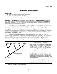
Fig. 1. Unconstrained solution for the polymer problem. 

450 

400 

350 

300 

250 

200 

150 

100 

50 

0 

0 2 4 6 8 10 

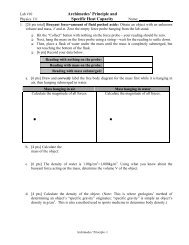
Fig. 2. Constrained solution for the polymer problem. 

tion. When asked to constrain the solution so that T p 6 400, each of the 

MATLAB solvers and VODE_F90 does so with at most a modest additional cost. 

The accompanying figures show the solutions obtained using both approaches 

for0 6 z 6 20. The constrained solution is preferable since it more closely 

resembles what is expected on physical grounds (Figs. 1 and 2).


6. Conclusion 

In Sections 3 and 4 we present an approach to imposing non-negativity constraints 

on the solutions of initial value problems for ODEs. It can be used for 

a wide range of methods found in the programs of [19] and VODE_F90. We 

present examples in Section 2 that explore the difficulties of the task and show 

in Section 5 that ourapproach can deal with all these difficulties in a satisfactory 

way. We note that the approach does not apply to the Rosenbrock method 

of ode23s and leave open the issue of applying non-negativity constraints 

when solving DAEs and fully implicit ODEs. 

References 

[1] R.C. Aiken (Ed.), Stiff Computation, Oxford University Press, Oxford, 1985. 

[2] K.E. Brenan, S.L. Campbell, L.R. Petzold, Numerical solution of initial-value problems in 

differential-algebraic equations, SIAM Classics in Applied Mathematics, vol. 14, SIAM, 

Philadelphia, 1996. 

[3] P.N. Brown, G.D. Byrne, A.C. Hindmarsh, VODE: A variable-coefficient ODE solver, SIAM 

J. Sci. Stat. Comput. 10 (1989) 1038–1051. 

[4] G. Buzzi Ferraris, D. Manca, BzzOde: a new C++ class of stiff and non-stiff ordinary 

differential equation systems, Comput. Chem. Eng. 22 (1998) 1595–1621. 

[5] G.D. Byrne, S. Thompson, A.C. Hindmarsh, VODE_F90: A Fortran 90 revision of VODE 

with added features, work in progress. 

[6] G. Dahlquist, L. Edsberg, G. Sköllermo, G. Söderlind, Are the numerical methods and 

software satisfactory for chemical kinetics? in: J. Hinze (Ed.), Numerical Integration of 

Differential Equations and Large Linear Systems, Lecture Notes in Math., vol. 968, Springer, 

New York, 1982, pp. 149–164. 

[7] L. Edsberg, Numerical methods for mass action kinetics, in: L. Lapidus, W.E. Schiesser 

(Eds.), Numerical Methods for Differential Systems, Academic, New York, 1976, pp. 181–195. 

[8] W.H. Enright, T.E. Hull, Comparing numerical methods for the solution of stiff systems of 

ODEs arising in chemistry, in: L. Lapidus, W.E. Schiesser (Eds.), Numerical Methods for 

Differential Systems, Academic, New York, 1976, pp. 48–66. 

[9] A.C. Hindmarsh, G.D. Byrne, Applications of EPISODE: an experimental package for the 

integration of systems of ordinary differential equations, in: L. Lapidus, W.E. Schiesser (Eds.), 

Numerical Methods for Differential Systems, Academic, New York, 1976, pp. 147–166. 

[10] G.R. Huxel, Private communication, Biology Dept., Univ. of South Florida, Tampa, FL, 

2004. 

[11] I. Karasalo, J. Kurylo, On solving the stiff ODEs of the kinetics of chemically reacting gas 

flow, Lawrence Berkeley Lab. Rept., Berkeley, CA, 1979. 

[12] MATLAB, The MathWorks, Inc., 3 Apple Hill Dr., Natick, MA 01760, 2004. 

[13] W.E. Schiesser, Private communication, Math. and Engr., Lehigh Univ., Bethlehem, PA, 2004. 

[14] W.E. Schiesser, Computational Mathematics in Engineering and Applied Science: ODEs, 

DAEs, and PDEs, CRC Press, Boca Raton, 1994. 

[15] L.F. Shampine, Conservation laws and the numerical solution of ODEs, Comp. Math. Appl. 

12B (1986) 1287–1296. 

[16] L.F. Shampine, Conservation laws and the numerical solution of ODEs, II, Comp. Math. 

Appl. 38 (1999) 61–72.


[17] L.F. Shampine, Numerical Solution of Ordinary Differential Equations, Chapman & Hall, 

New York, 1994. 

[18] L.F. Shampine, M.E. Hosea, Analysis and implementation of TR-BDF2, Appl. Numer. Math. 

20 (1996) 21–37. 

[19] L.F. Shampine, M.W. Reichelt, The MATLAB ODE Suite, SIAM J. Sci. Comput. 18 (1997) 1– 

22.

Non-negative solutions of ODEs - Radford University

Create successful ePaper yourself

Delete template?

Save as template?