Parametric Curves and Polar Coordinates
Parametric Curves and Polar Coordinates
Parametric Curves and Polar Coordinates

You also want an ePaper? Increase the reach of your titles
YUMPU automatically turns print PDFs into web optimized ePapers that Google loves.
<strong>Parametric</strong> <strong>Curves</strong> <strong>and</strong> <strong>Polar</strong> <strong>Coordinates</strong><br />
Math 251, Fall 2011<br />
J. Gerlach<br />
<strong>Parametric</strong> <strong>Curves</strong><br />
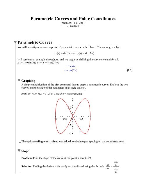
We will investigate several aspects of parametric curves in the plane. The curve given by<br />
<strong>and</strong><br />
will serve as an example throughout, <strong>and</strong> we begin by defining the curve once <strong>and</strong> for all.<br />
(1.1)<br />
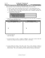
Graphing<br />
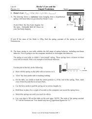
A simple modification of the plot comm<strong>and</strong> lets us graph a parametric curve: Enclose the two<br />
curves <strong>and</strong> the range of the parameter in a single bracket.<br />
1<br />
0 1<br />
The option scaling=constrained was added to obtain equal spacing on the coordinate axes.<br />
Slope<br />
Problem:<br />
Solution: Finding the derivative is easily accomplished using the formula .
(1.2.1)<br />
(1.2.3)<br />
Thus the slope at is -2.<br />
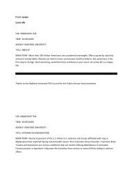
Graph of the <strong>Parametric</strong> Curve with a Tangent Line<br />
Problem: in a common<br />
figure.<br />
Solution: The solution requires several steps. First we denote the point which corresponds to t=<br />
(1.3.1)<br />
that m was determined above)<br />
(1.3.2)<br />
Thus the tangent line has slope m=-2.<br />
(1.3.3)<br />
We have several options to obtain the curve <strong>and</strong> the tangent line in a common figure. For one we<br />
could plot the curve <strong>and</strong> the tangent line separately <strong>and</strong> then superimpose the two with the<br />
display comm<strong>and</strong>. This approach requires uploading the plots package, <strong>and</strong> we will not apply this<br />
method here. As an alternative we can express the tangent line in parametric form <strong>and</strong> plot the<br />
two curves simultaneously, <strong>and</strong> we will take this route. A third option will be shown below.
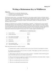
The tangent line y -Y = M(x-X) can be expressed in parametric form by setting x = t, <strong>and</strong> we get<br />
y = Y +M(t-X)<br />
This formula can be directly substituted into the plotting comm<strong>and</strong>. Result:<br />
1<br />
0 1<br />
Note that in the plotting comm<strong>and</strong> the two parametric curves were enclosed by brackets <strong>and</strong> that<br />
the comm<strong>and</strong> has the structure plot( [ [first curve] , [second curve] ], options);<br />
The third option is more elegant. We compute the tangent lines for the two functions x(t) <strong>and</strong> y(t)<br />
curve. Here are the details:<br />
(1.3.4)<br />
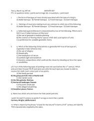
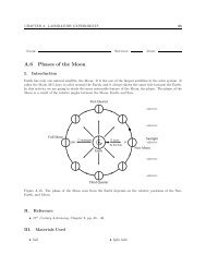
The next two pictures show that we indeed calculated ordinary tangent lines.<br />
(1.3.5)<br />
1<br />
0<br />
0 1 2 3<br />
t
1<br />
0<br />
1 2 3<br />
t<br />
Viewed as parametric curve, the pair lx(t) <strong>and</strong> ly(t) becomes the tangent line of our curve.<br />
1<br />
0 1<br />
Find Points with a Given Slope<br />
Problem: Find the point in the first quadrant where the slope equals -1.<br />
Solution: We set the slope dy/dx = m, <strong>and</strong> solve the equation m=-1 for t.<br />
(1.4.1)<br />
(1.4.2)<br />
The first value appears to be the desired value for t, <strong>and</strong> we name it T (copy-<strong>and</strong>-paste)<br />
(1.4.3)
Then the point with slope m=-1 is located at x(T) <strong>and</strong> y(T). These points are<br />
(1.4.4)<br />
(1.4.5)<br />
Numerically the coordinates of the point with slope -1 are<br />
0.8660254040<br />
0.9550219348<br />
Clearly, this point belongs to the first quadrant.<br />
(1.4.6)<br />
Find the Slopes at the Origin<br />
Problem: What are the slopes as the curve passes through the origin?<br />
Solution: First we need to find the value of the parameter when the curve passes through the<br />
origin, that is, we must solve x(t)=0 <strong>and</strong> y(t)= 0 simultaneously.<br />
We find two values. Check:<br />
(1.5.1)<br />
For the slopes we find:<br />
(1.5.2)<br />
2<br />
(1.5.3)<br />
Thus the slopes are +2 <strong>and</strong> -2.<br />
(1.5.4)<br />
Arc Length<br />
Problem: What is the arc length of the curve?<br />
Solution: We can implement the arc length formula directly, <strong>and</strong> we obtain using the templates on<br />
the left<br />
(1.6.1)
at 5 digits<br />
9.4294<br />
Maple couldn't find an analytic solution, <strong>and</strong> we accept a numerical approximation in its place.<br />
Area<br />
Problem: Find the area enclosed by the curve.<br />
Solution: The area between a parametric curve <strong>and</strong> the x-axis can be computed as follows:<br />
where <strong>and</strong> are to be selected to match the endpoints.<br />
In our example we use symmetry, <strong>and</strong> multiply the area in the first quadrant by 4 to get the total<br />
8<br />
3<br />
(1.7.1)<br />
<strong>Polar</strong> <strong>Coordinates</strong><br />
curve. First, we define r once <strong>and</strong> for all<br />
(2.1)<br />
(2.2)<br />
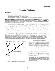
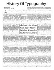
<strong>Polar</strong> Graphs<br />
Plotting in polar coordinates requires the option coords=polar, everything else is pretty much the<br />
same. This is the equivalent of setting your calculator to the polar function mode. Here is the<br />
graph:
8<br />
7<br />
6<br />
5<br />
4<br />
3<br />
2<br />
1<br />
0 1 2 3 4<br />
The plots package offers a nice alternative. In order to use it, we need to activate it first with the<br />
comm<strong>and</strong><br />
Use a colon to avoid unnecessary output. Now we are ready to plot.<br />
2<br />
4<br />
4<br />
0 1 2 3 4 5 6 7 0<br />
4<br />
4<br />
2<br />
Slope at a Given Point<br />
Problem: What is the slope of the curve at the point (x,y)=(3,0)?<br />
Solution:<br />
dy/dx we follow the usual procedure for parametric curves, this time with the diff comm<strong>and</strong><br />
(2.2.1)
(2.2.2)<br />
And now we set t = 0<br />
(2.2.3)<br />
Thus the desired slope is 3/5.<br />
3<br />
5<br />
(2.2.4)<br />
Graph of the <strong>Polar</strong> Curve with a Tangent Line<br />
Problem: Graph the curve along with its tangent line at the point (3,0) in a common figure.<br />
Solution: We know from the last problem that the slope is 3/5, <strong>and</strong> using the point-slope form of a<br />
line, the tangent line is given by<br />
For the graph we have two alternatives: Either express the line in polar coordinates <strong>and</strong> use a<br />
single ploting statement, or graph the two pieces separately <strong>and</strong> superimpose the graphs. We will<br />
demonstrate both.<br />
In polar coordinates the line becomes<br />
<strong>and</strong> solving this equation for r we find<br />
(2.3.1)<br />
(2.3.2)<br />
This is an expression for the tangent line in polar coordinates, <strong>and</strong> with a simple copy-<strong>and</strong>-paste<br />
we obtain
8<br />
6<br />
4<br />
2<br />
0 2 4 6<br />
The alternative requires the plotting package (which is already activated).<br />
2<br />
4<br />
4<br />
0 1 2 3 4 5 6 7<br />
x<br />
0<br />
4<br />
4<br />
2<br />
Slopes at the Origin<br />
Problem: What are the slopes of the curve as it passes though the origin?<br />
Solution: First we set r=0 to find the points where the curve passes through the origin.<br />
(2.4.1)<br />
This result is of limited use. But applying our knowledge of trigonometry we conclude that r(t)=0
for<br />
Let's confirm this:<br />
0<br />
(2.4.2)<br />
Now we calculate the slope at these points.<br />
0<br />
(2.4.3)<br />
(2.4.4)<br />
(2.4.5)<br />
3<br />
4<br />
(2.4.6)<br />
(2.4.7)<br />
(2.4.8)<br />
There is a Much easier way to determine the slope. We know from class that the slope is the<br />
tangent of the respective angles.<br />
3<br />
4<br />
(2.4.9)
Arc Length<br />
Problem: Find the arc length of the curve.<br />
Solution: Here we implement the familiar formula for the arc length of a polar curve directly, <strong>and</strong><br />
let maple do the work.<br />
(2.5.1)<br />
at 10 digits<br />
34.31368713<br />
(2.5.2)<br />
The result involves special functions, but numerical evaluation leads to an acceptable result.<br />
Area<br />
Problem: Compute the area enclosed by the inner loop of the curve.<br />
Solution: The inner part of the curve is traced when T1 < t < T2 (the numbers T1 <strong>and</strong> T2 were<br />
found above). Using the area formula for polar curves we find that<br />
(2.6.1)<br />
The area is roughly two square units.<br />
1.93684719<br />
(2.6.2)