Computing Fixed Points and Cycles for the Discrete Logistic Equation
Computing Fixed Points and Cycles for the Discrete Logistic Equation
Computing Fixed Points and Cycles for the Discrete Logistic Equation

Create successful ePaper yourself
Turn your PDF publications into a flip-book with our unique Google optimized e-Paper software.
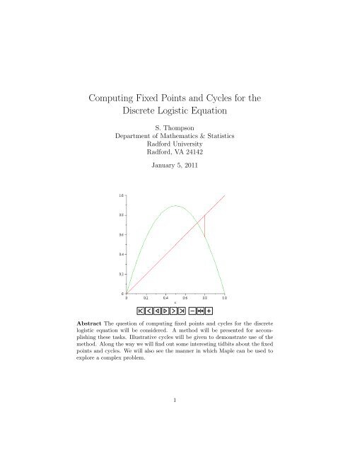
<strong>Computing</strong> <strong>Fixed</strong> <strong>Points</strong> <strong>and</strong> <strong>Cycles</strong> <strong>for</strong> <strong>the</strong><br />
<strong>Discrete</strong> <strong>Logistic</strong> <strong>Equation</strong><br />
S. Thompson<br />
Department of Ma<strong>the</strong>matics & Statistics<br />
Rad<strong>for</strong>d University<br />
Rad<strong>for</strong>d, VA 24142<br />
January 5, 2011<br />
Abstract The question of computing fixed points <strong>and</strong> cycles <strong>for</strong> <strong>the</strong> discrete<br />
logistic equation will be considered. A method will be presented <strong>for</strong> accomplishing<br />
<strong>the</strong>se tasks. Illustrative cycles will be given to demonstrate use of <strong>the</strong><br />
method. Along <strong>the</strong> way we will find out some interesting tidbits about <strong>the</strong> fixed<br />
points <strong>and</strong> cycles. We will also see <strong>the</strong> manner in which Maple can be used to<br />
explore a complex problem.<br />
1
1 Introduction<br />
We are interested in <strong>the</strong> task of computing fixed points <strong>and</strong> N-cycles <strong>for</strong> <strong>the</strong><br />
well known <strong>and</strong> much studied discrete logistic equation<br />
x n+1 = kx n (1 − x n ) (1)<br />
where k is a constant satisfying 0 ≤ k ≤ 4. We are particularly interested in<br />
values of k between 3 <strong>and</strong> 4. Background <strong>and</strong> a detailed discussion of Eq. (1)<br />
may be found in [3]. A delightful elementary introduction may be found in [1];<br />
<strong>and</strong> a more detailed ma<strong>the</strong>matical treatment may be found in [2].<br />
Finding N-cycles entails finding <strong>the</strong> fixed points of F N (x), <strong>the</strong> Nth composition<br />
of <strong>the</strong> function<br />
F (x) = kx(1 − x) (2)<br />
with itself. We thus must find <strong>the</strong> solutions of<br />
F N (x) = x. (3)<br />
We must <strong>the</strong>n determine <strong>the</strong> N-cycles determined by <strong>the</strong> fixed points. We are<br />
interested primarily in “true” (prime in <strong>the</strong> terminology of [3]) N-cycles, ones<br />
<strong>for</strong>ming a sequence x 0 , . . . , x N−1 where x 0 is a solution of Eq. (3), F (x N−1 ) =<br />
x 0 , <strong>and</strong> N − 1 is <strong>the</strong> first value <strong>for</strong> which <strong>the</strong> latter occurs. This is in general a<br />
<strong>for</strong>midable task since F N (x) is a polynomial of degree 2 N . While it is possible<br />
to use tools available in a Computer Algebra System (CAS) such as Maple 11<br />
[4] to find <strong>the</strong> fixed points <strong>and</strong> corresponding cycles directly <strong>for</strong> relatively small<br />
values of N, say, N < 5, it is effectively not possible to do so <strong>for</strong> larger values<br />
of N. We will describe a method that we have used to help Maple accomplish<br />
<strong>the</strong>se tasks <strong>for</strong> values of N up to 15 <strong>and</strong> <strong>for</strong> general values of k. From our<br />
discussion, it should become clear that constructing cycles without <strong>the</strong> use of a<br />
CAS such as Maple is simply intractable even <strong>for</strong> small values on N.<br />
We note that cobweb diagrams [1] are used to display N-cycles (more generally,<br />
<strong>the</strong>y are to depict <strong>the</strong> iterates <strong>for</strong> any sequence). These diagrams depict<br />
<strong>the</strong> relevant fixed points along with <strong>the</strong> graphs of y = F (x) <strong>and</strong> <strong>the</strong> line<br />
y = x. Starting from a fixed point, locate <strong>the</strong> corresponding point on <strong>the</strong> curve<br />
y = F (x). Then locate <strong>the</strong> corresponding point on <strong>the</strong> line y = x. Repeat this<br />
process to follow <strong>the</strong> <strong>for</strong>mation of <strong>the</strong> N-cycle. This process is illustrated in <strong>the</strong><br />
animated gif files attachments that are mentioned later in this paper.<br />
It should be noted that our approach is somewhat empirical. However, <strong>the</strong><br />
onset values of k at which cycles of length 1-8 first appear can be determined<br />
analytically. (See [6] <strong>and</strong> <strong>the</strong> references <strong>the</strong>rein). In each such case, we were<br />
able to find cycles of <strong>the</strong> desired length <strong>for</strong> each of <strong>the</strong>se onset values. We<br />
experimented to approximate <strong>the</strong> onset values <strong>for</strong> cycles of length 9-12. (Refer<br />
to <strong>the</strong> attached Maple worksheet <strong>for</strong> <strong>the</strong> approximate onset values we obtained.<br />
The worksheet also contains a summary of <strong>the</strong> numbers of cycles of length N<br />
that we were able to locate <strong>for</strong> different values of k.) To get an idea of where to<br />
start looking <strong>for</strong> cycles of <strong>the</strong>se lengths, we used Sharkovskii’s Theorem [2]-[3]<br />
2
(which involves ordering <strong>the</strong> natural numbers in a manner such that if any cycle<br />
of length N exists, all successors in <strong>the</strong> ordering also yield cycles of length N).<br />
Each of <strong>the</strong> cycles reported in this paper is consistent with Sharkovskii’s ordering<br />
<strong>and</strong> with <strong>the</strong> onset values <strong>for</strong> shorter cycles. As a matter of interest, we fur<strong>the</strong>r<br />
note that certain values of k yield cycles of several lengths. For example, k = 3.9<br />
yields cycles of length 2-12 <strong>and</strong> k = 3.75 yields cycles of length 2-10. Finally,<br />
we note that it is instructive to use <strong>the</strong> attached worksheet to experiment with<br />
values on each side of <strong>the</strong> onset values to see how <strong>the</strong> cycles with longer lengths<br />
appear.<br />
2 The Easiest Case, k = 4<br />
Though <strong>the</strong> title of this section may seem surprising to readers familiar with<br />
<strong>the</strong> complexity of <strong>the</strong> logistic equation, <strong>the</strong> easiest case to h<strong>and</strong>le occurs when<br />
k = 4. In this case, Eq. (3) has precisely 2 N real fixed points <strong>and</strong> N-cycles exist<br />
<strong>for</strong> each N. It is instructive to consider <strong>the</strong> manner in which <strong>the</strong> fixed points<br />
arise <strong>for</strong> this value of k.<br />
Graphs of F 1 (x), F 2 (x), <strong>and</strong> F 3 (x) suggest <strong>the</strong>re are precisely 2 N fixed points<br />
<strong>for</strong> each value of N <strong>and</strong> it suggests how we might go about finding <strong>the</strong> fixed<br />
points of F N (x). A simple calculation shows that <strong>the</strong> following hold<br />
F N+1 (x) = 4F N (x) (1 − F N (x)) (4)<br />
F ′ N+1(x) = 4F ′ N (x) (1 − 2F N (x)) (5)<br />
Eq. (4) <strong>and</strong> Eq. (5) may be used to show that <strong>the</strong> zeroes of F N+1 (x) = 0 consist<br />
of <strong>the</strong> zeroes of F N (x) = 0 along with new values determined by F N (x) = 1.<br />
The values <strong>for</strong> which F N+1 (x) = 1 are <strong>the</strong> values <strong>for</strong> which F N (x) = 1 2 ; <strong>and</strong><br />
<strong>the</strong> zeroes of F N+1 (x) = 0 thus consist of 0 <strong>and</strong> 1 along with 2 N − 2 zeroes<br />
with multiplicity 2. Each of <strong>the</strong> intervals with <strong>the</strong>se distinct zeroes as endpoints<br />
contains exactly two fixed points of F N+1 (x). As an example, <strong>the</strong> zeroes of<br />
F 1 (x) are 0 <strong>and</strong> 1. (Alternatively, <strong>the</strong> intervals between successive points with<br />
F N ′ (x) = 0 each contain one fixed point.) These two values give rise to 0, 1 2 ,<br />
1<br />
2 , <strong>and</strong> 1 as <strong>the</strong> zeroes of F 2(x). These four values in turn yield <strong>the</strong> zeroes of<br />
F 3 (x) consisting of <strong>the</strong>se four values along with <strong>the</strong> two multiplicity 2 values<br />
1<br />
2<br />
+<br />
−<br />
√<br />
2<br />
4<br />
. The corresponding intervals each contain <strong>the</strong> two fixed points that can<br />
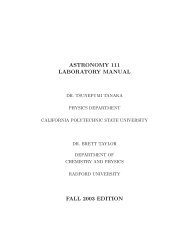
be located by subdividing <strong>the</strong> interval twice. Using <strong>the</strong> Maple solve comm<strong>and</strong><br />
<strong>for</strong> N = 2 yields <strong>the</strong> fixed points x = 0, x = 3 4 , <strong>and</strong> x = 5 +<br />
8 − 8√ 1 5. For N = 3<br />
it yields <strong>the</strong> fixed points (rounded <strong>for</strong> display purposes) 0, 0.11698, 0.18826,<br />
0.41318, 0.61126, 0.75, 0.95048, <strong>and</strong> 0.96985. Figure 1 depicts a 2-cycle <strong>and</strong> a<br />
3-cycle determined by <strong>the</strong>se fixed points.<br />
In principle, <strong>the</strong> Maple solve comm<strong>and</strong> can be used to solve <strong>the</strong> necessary<br />
polynomial equations in <strong>the</strong> above procedure. Un<strong>for</strong>tunately, <strong>for</strong> values of N as<br />
small as 4 or 5, use of <strong>the</strong> solve comm<strong>and</strong> is unsuccessful in some cases <strong>and</strong><br />
in o<strong>the</strong>r cases an incorrect number of solutions is found. Use of <strong>the</strong> numeric<br />
fsolve comm<strong>and</strong> leads to similar results since fsolve recognizes a polynomial<br />
3
as a “known” function <strong>and</strong> employs symbolic procedures to solve polynomial<br />
equations. Difficulties using solve <strong>and</strong> fsolve led us to explore o<strong>the</strong>r ways to<br />
determine <strong>the</strong> fixed points. An alternate way to find <strong>the</strong> fixed points without<br />
directly solving polynomial equations is described in <strong>the</strong> next section.<br />
(a)<br />
1.0 (b)<br />
1.0<br />
0.8<br />
0.8<br />
0.6<br />
0.6<br />
0.4<br />
0.4<br />
0.2<br />
0.2<br />
0<br />
0 0.2 0.4 0.6 0.8 1.0<br />
x<br />
0<br />
0 0.2 0.4 0.6 0.8 1.0<br />
x<br />
Figure 1: 2-cycle <strong>and</strong> 3-cycle <strong>for</strong> k = 4<br />
3 Backward Compositions<br />
If x = F n (x) <strong>the</strong>n we may solve <strong>the</strong> equation x = kx n−1 (1 − x n−1 ) <strong>for</strong> <strong>the</strong> two<br />
values x n−1 <strong>for</strong> which F (x n−1 ) = x. We refer to <strong>the</strong>se two values as ancestors<br />
of x. (They are sometimes referred to as predecessors or preimages of x.) These<br />
values are given by<br />
(<br />
) √1 − 4 k x<br />
x n−1 = 1 2<br />
1 + −<br />
. (6)<br />
Let us <strong>the</strong>n define <strong>the</strong> functions<br />
(<br />
)<br />
g 0 (x) = 1 1 −<br />
√1 − 4 2<br />
k x<br />
(<br />
)<br />
g 1 (x) = 1 1 +<br />
√1 − 4 2<br />
k x<br />
(7)<br />
(8)<br />
For a given value of x, g 0 (x) <strong>and</strong> g 1 (x) yield <strong>the</strong> two immediate ancestors of x.<br />
The four ancestors of <strong>the</strong>se values are given by <strong>the</strong> compositions g 0 ◦ g 0 (x n−1 ),<br />
g 0 ◦g 1 (x n−1 ), g 1 ◦g 0 (x n−1 ), <strong>and</strong> g 1 ◦g 1 (x n−1 ). Continuing in this fashion we can<br />
locate <strong>the</strong> 2 N ancestors of x. We can <strong>the</strong>n locate <strong>the</strong> fixed points of x = F N (x)<br />
by solving <strong>the</strong> equations<br />
x = Φ(x) (9)<br />
4
where Φ(x) is any of <strong>the</strong> 2 N nested square root compositions<br />
g i0 ◦ · · · ◦ g iN (x)<br />
<strong>and</strong> each i j is 0 or 1 since any such solution satisfies Eq. (3). To locate <strong>the</strong> zeroes<br />
of <strong>the</strong> functions, we used a Maple adaptation Zeromw of <strong>the</strong> well-known Zero<br />
root finder [5] which uses a combination of <strong>the</strong> secant method <strong>and</strong> bisection.<br />
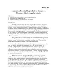
Although <strong>the</strong> fixed points of F N (x) become closely spaced <strong>for</strong> increasing N,<br />
<strong>the</strong>y are well-separated by <strong>the</strong> above functions <strong>and</strong> are located easily. Figure 2<br />
depicts a 6-cycle <strong>for</strong> k = 4. We obtained similar N-cycles <strong>for</strong> larger values of N.<br />
(Values of N in <strong>the</strong> range 12–15 were as large as our computer was willing to<br />
tolerate.) None are displayed here because higher order cycles look very much<br />
like <strong>the</strong> displayed 6-cycle due to <strong>the</strong> fact that some of <strong>the</strong> cycle points tend to<br />
cluster near 0 <strong>and</strong> 1 making it hard to distinguish between <strong>the</strong>m in <strong>the</strong> plotted<br />
cycles.<br />
1.0<br />
0.8<br />
0.6<br />
0.4<br />
0.2<br />
0<br />
0 0.2 0.4 0.6 0.8 1.0<br />
x<br />
Figure 2: 6-cycle <strong>for</strong> k = 4<br />
Note that when k = 4 <strong>the</strong> domain of each of <strong>the</strong> backward compositions is<br />
<strong>the</strong> interval [0, 1]. This is as good as it gets. In general, <strong>the</strong> real domains of <strong>the</strong><br />
functions Φ(x) are subsets of this interval, that is, some of <strong>the</strong> ancestors of x are<br />
complex. The key to making our approach work is to find <strong>the</strong>se real domains<br />
so that we can locate <strong>the</strong> real ancestors of x. This will be discussed fur<strong>the</strong>r in<br />
<strong>the</strong> next section.<br />
4 Backward Composition Domains<br />
In order to find a real fixed point x using <strong>the</strong> procedure described above, x<br />
must belong to <strong>the</strong> domain of each of <strong>the</strong> nested square root functions used to<br />
build Φ(x). For g 0 (x) <strong>and</strong> g 1 (x) to be real, we must have x ≤ x 0 = k 4 . An<br />
interesting thing happens when we consider <strong>the</strong> cut points at which successive<br />
discriminants are equal to 0. Compositions of length two lead to <strong>the</strong> cut point<br />
x 1 = x 0<br />
(1 − (2x 0 − 1) 2) . (10)<br />
5
Continuing with successively higher order compositions, we inductively find <strong>the</strong><br />
sequence of cut points satisfying<br />
x j = x j−1<br />
(1 − (2x j−1 − 1) 2) , j = 1, . . . , N − 1 (11)<br />
A simple calculation shows that<br />
x j = kx j−1 (1 − x j−1 ) , (12)<br />
That is, <strong>the</strong> cut points are <strong>the</strong> first N terms of a logistic sequence with initial<br />
iterate equal to k 4<br />
. This, perhaps surprising, tidbit is quite useful. The domains<br />
of each of <strong>the</strong> Φ(x) functions are (single) intervals of <strong>the</strong> <strong>for</strong>m [a, b] where a <strong>and</strong><br />
b are two elements of this sequence with a < b or of <strong>the</strong> <strong>for</strong>m [a, b] where a = 0<br />
<strong>and</strong> b is an element of <strong>the</strong> cut sequence. For k = 4 note that <strong>the</strong> sequence is<br />
1, 0, 0, . . . leading to <strong>the</strong> interval [0, 1] as <strong>the</strong> domain <strong>for</strong> each Φ(x). For o<strong>the</strong>r<br />
values of k, some of <strong>the</strong> cut points may be close toge<strong>the</strong>r <strong>and</strong> in some cases <strong>the</strong><br />
real domain of a particular composition degenerates to a single point. This is<br />
one reason it is necessary to locate <strong>the</strong> cut points since some of <strong>the</strong> fixed points<br />
tend to cluster in <strong>the</strong>se small intervals.<br />
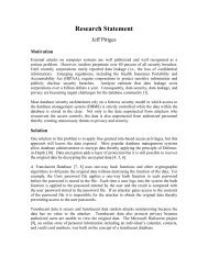
Although it is relatively easy to obtain N-cycles <strong>for</strong> a good many values<br />
of N <strong>and</strong> k, our procedure has two drawbacks. It requires <strong>the</strong> solution of<br />
2 N nonlinear equations making it impractical <strong>for</strong> large values of N due to <strong>the</strong><br />
exponentially increasing complexity of <strong>the</strong> calculations. However, we have used<br />
it to locate cycles <strong>for</strong> many values of k <strong>and</strong> values of N up to 15 (although<br />
in some cases <strong>the</strong> calculation times <strong>for</strong> N > 12 are quite long). Figures 3–8<br />
represent a miscellaneous sample of cycles of various lengths 2–13. A second<br />
nasty drawback can occur even <strong>for</strong> some small values of N. Unlike <strong>the</strong> case<br />
k = 4, it is necessary in some cases to subdivide <strong>the</strong> domains more than twice<br />
in order to find bracketing intervals containing <strong>the</strong> fixed points. In most cases<br />
2–10 subdivisions are sufficient but in some situations many more subdivisions<br />
are required. The cases we have in mind are <strong>the</strong> ones near <strong>the</strong> “onset” values<br />
of k discussed in <strong>the</strong> next section.<br />
5 Onset Values of k<br />
Since Zeromw requires a sign change to locate zeroes, success of <strong>the</strong> procedure<br />
described above depends on being able to subdivide <strong>the</strong> domains of <strong>the</strong> composition<br />
functions to obtain bracketing intervals <strong>for</strong> <strong>the</strong> fixed points. In some cases,<br />
our procedure is inefficient in locating zeroes with multiplicity greater than 1 or<br />
<strong>for</strong> nearby values of k <strong>for</strong> which <strong>the</strong>re are very closely spaced zeroes near such a<br />
zero with multiplicity greater than 1. Such zeroes occur <strong>for</strong> special onset values<br />
of k at which cycles of longer lengths originate. Several such onset values are<br />
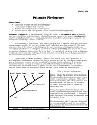
known (see [6] <strong>and</strong> <strong>the</strong> links cited <strong>the</strong>rein). Figures 9–12 depict cycles of length<br />
3–8 corresponding to <strong>the</strong>se onset values. Each cycle depicted was obtained by<br />
rounding <strong>the</strong> 54th digit of <strong>the</strong> corresponding exact value of k upward. This was<br />
6
(a)<br />
0.7<br />
0.6<br />
0.5<br />
0.4<br />
0.3<br />
0.2<br />
0.1<br />
0<br />
0 0.1 0.2 0.3 0.4 0.5 0.6 0.7<br />
x<br />
(b)<br />
0.9<br />
0.8<br />
0.7<br />
0.6<br />
0.5<br />
0.4<br />
0.3<br />
0.2<br />
0.1<br />
0<br />
0 0.1 0.2 0.3 0.4 0.5 0.6 0.7 0.8 0.9<br />
x<br />
Figure 3: (a) 2-cycle <strong>for</strong> k = 3.1 (b) 3-cycle <strong>for</strong> k = 3.83<br />
(a)<br />
0.8<br />
(b)<br />
0.9<br />
0.7<br />
0.6<br />
0.5<br />
0.4<br />
0.8<br />
0.7<br />
0.6<br />
0.5<br />
0.4<br />
0.3<br />
0.3<br />
0.2<br />
0.2<br />
0.1<br />
0.1<br />
0<br />
0 0.1 0.2 0.3 0.4 0.5 0.6 0.7 0.8<br />
x<br />
0<br />
0 0.1 0.2 0.3 0.4 0.5 0.6 0.7 0.8 0.9<br />
x<br />
Figure 4: (a) 4-cycle <strong>for</strong> k = 3.5 (b) 5-cycle <strong>for</strong> k = 3.83<br />
done <strong>for</strong> convenience <strong>and</strong> since <strong>for</strong> some values of k, <strong>the</strong>re is no true cycle of <strong>the</strong><br />
desired length except <strong>for</strong> values of k strictly larger than <strong>the</strong> onset value.<br />
We should note that h<strong>and</strong>ling <strong>the</strong> k = 3 onset value <strong>for</strong> 2-cycles in this<br />
manner was unsuccessful. Use of <strong>the</strong> method is prohibitive <strong>for</strong> smaller values<br />
of k near k = 3 due to <strong>the</strong> number of required subdivisions of <strong>the</strong> composition<br />
domains. However, in <strong>the</strong> Maple worksheet we used, it is possible to reduce <strong>the</strong><br />
size of <strong>the</strong> composition domains if additional in<strong>for</strong>mation is available. (Such<br />
in<strong>for</strong>mation may be obtained by inspecting plots of <strong>the</strong> functions used in <strong>the</strong><br />
root finding.) k = 3.000000001 was <strong>the</strong> smallest value of k <strong>for</strong> which we bo<strong>the</strong>red<br />
to do this in order to compute a true 2-cycle. Since <strong>the</strong> solve comm<strong>and</strong> is able<br />
to find <strong>the</strong> fixed points of F 2 (x) <strong>for</strong> values of k near 3, it does a more satisfactory<br />
job finding <strong>the</strong> relevant fixed points than does <strong>the</strong> present method <strong>for</strong> values of<br />
k slightly larger than 3. We should also note that we were able to use <strong>the</strong> Maple<br />
factor to find <strong>the</strong> fixed points <strong>and</strong> onset cycles <strong>for</strong> <strong>the</strong>se values of k (albeit at<br />
7
(a)<br />
0.9<br />
0.8<br />
0.7<br />
0.6<br />
0.5<br />
0.4<br />
0.3<br />
0.2<br />
0.1<br />
0<br />
0 0.1 0.2 0.3 0.4 0.5 0.6 0.7 0.8 0.9<br />
x<br />
(b)<br />
0.9<br />
0.8<br />
0.7<br />
0.6<br />
0.5<br />
0.4<br />
0.3<br />
0.2<br />
0.1<br />
0<br />
0 0.1 0.2 0.3 0.4 0.5 0.6 0.7 0.8 0.9<br />
x<br />
Figure 5: (a) 6-cycle <strong>for</strong> k = 1 + √ 8 (b) 7-cycle <strong>for</strong> k = 3.85<br />
(a)<br />
0.8<br />
0.7<br />
0.6<br />
0.5<br />
0.4<br />
0.3<br />
0.2<br />
0.1<br />
0<br />
0 0.1 0.2 0.3 0.4 0.5 0.6 0.7 0.8<br />
x<br />
(b)<br />
0.9<br />
0.8<br />
0.7<br />
0.6<br />
0.5<br />
0.4<br />
0.3<br />
0.2<br />
0.1<br />
0<br />
0 0.1 0.2 0.3 0.4 0.5 0.6 0.7 0.8 0.9<br />
x<br />
Figure 6: (a) 8-cycle <strong>for</strong> k = 3.55 (b) 9-cycle <strong>for</strong> k = 3.9<br />
considerably more expense). The precise values of k used to produce <strong>the</strong> o<strong>the</strong>r<br />
onset cycles depicted in Figures 9–12 were:<br />
3-cycle:<br />
3.82842712474619009760337744841939615713934375075389615<br />
4-cycle:<br />
3.44948974278317809819728407470589139196594748065667013<br />
5-cycle:<br />
3.73817237526596236943026155967953197344411544048999193<br />
6-cycle:<br />
3.62655316169497372587723225209331749170947578579502470<br />
7-cycle:<br />
3.70164076416034958182464378984088922014429158951520644<br />
8-cycle:<br />
8
(a)<br />
0.9<br />
0.8<br />
0.7<br />
0.6<br />
0.5<br />
0.4<br />
0.3<br />
0.2<br />
0.1<br />
0<br />
0 0.1 0.2 0.3 0.4 0.5 0.6 0.7 0.8 0.9<br />
x<br />
(b)<br />
0.9<br />
0.8<br />
0.7<br />
0.6<br />
0.5<br />
0.4<br />
0.3<br />
0.2<br />
0.1<br />
0<br />
0 0.1 0.2 0.3 0.4 0.5 0.6 0.7 0.8 0.9<br />
x<br />
Figure 7: (a) 10-cycle <strong>for</strong> k = 3.85 (b) 11-cycle <strong>for</strong> k = 3.85<br />
(a)<br />
0.9<br />
0.8<br />
0.7<br />
0.6<br />
(b)<br />
0.9<br />
0.8<br />
0.7<br />
0.6<br />
0.5<br />
0.5<br />
0.4<br />
0.4<br />
0.3<br />
0.3<br />
0.2<br />
0.2<br />
0.1<br />
0.1<br />
0<br />
0 0.1 0.2 0.3 0.4 0.5 0.6 0.7 0.8 0.9<br />
x<br />
0<br />
0 0.1 0.2 0.3 0.4 0.5 0.6 0.7 0.8 0.9<br />
x<br />
Figure 8: (a) 12-cycle <strong>for</strong> k = 3.9 (b) 13-cycle <strong>for</strong> k = 3.7<br />
3.54409035955192285361596598660480454058309984544457368<br />
Though somewhat more cumbersome (due to having to deal appropriately<br />
with poles), we found it possible to also produce <strong>the</strong>se cycles in a different way.<br />
By replacing <strong>the</strong> equation x − Φ(x) = 0 with<br />
x − Φ(x)<br />
1 − Φ ′ (x) = 0 (13)<br />
it was possible to locate higher multiplicity zeroes <strong>and</strong> very closely spaced zeroes<br />
using far fewer subdivisions of <strong>the</strong> composition domains. The cycles depicted in<br />
Figures 9–12 were obtained in this manner.<br />
9
(a)<br />
0.7<br />
0.6<br />
0.5<br />
0.4<br />
0.3<br />
0.2<br />
0.1<br />
0<br />
0 0.1 0.2 0.3 0.4 0.5 0.6 0.7<br />
x<br />
(b)<br />
0.9<br />
0.8<br />
0.7<br />
0.6<br />
0.5<br />
0.4<br />
0.3<br />
0.2<br />
0.1<br />
0<br />
0 0.1 0.2 0.3 0.4 0.5 0.6 0.7 0.8 0.9<br />
x<br />
Figure 9: (a) Onset 2-cycle <strong>for</strong> k = 3 (b) Onset 3-cycle <strong>for</strong> k = 3.828<br />
(a)<br />
0.8<br />
0.7<br />
0.6<br />
0.5<br />
0.4<br />
(b)<br />
0.9<br />
0.8<br />
0.7<br />
0.6<br />
0.5<br />
0.4<br />
0.3<br />
0.3<br />
0.2<br />
0.2<br />
0.1<br />
0.1<br />
0<br />
0 0.1 0.2 0.3 0.4 0.5 0.6 0.7 0.8<br />
x<br />
0<br />
0 0.1 0.2 0.3 0.4 0.5 0.6 0.7 0.8 0.9<br />
x<br />
Figure 10: (a) Onset 4-cycle <strong>for</strong> k = 3.449 (b) Onset 5-cycle <strong>for</strong> k = 3.738<br />
6 Suggested Student Explorations<br />
The logistic equation is rife with interesting properties that beg to be investigated.<br />
Following are a few interesting questions that students might wish to<br />
explore.<br />
6.1 Question 1<br />
To develop an appreciation <strong>for</strong> <strong>the</strong> manner in which cycles of longer length develop<br />
near <strong>the</strong> onset values of k, you might wish to study <strong>the</strong> following cycles.<br />
Figure 13 depicts a 4-cycle <strong>for</strong> k = 3.54 <strong>and</strong> an 8-cycle <strong>for</strong> k = 3.55. Note how<br />
<strong>the</strong> additional close zeroes in <strong>the</strong> latter cycle get into <strong>the</strong> act <strong>and</strong> prevent a<br />
4-cycle from <strong>for</strong>ming. Animated versions of <strong>the</strong>se cycles follow Figure 13. Depending<br />
on what is displayed, you need only play <strong>the</strong> cycle <strong>for</strong>ward or backward<br />
10
(a)<br />
0.9 (b)<br />
0.8<br />
0.7<br />
0.6<br />
0.5<br />
0.4<br />
0.3<br />
0.2<br />
0.1<br />
0<br />
0 0.1 0.2 0.3 0.4 0.5 0.6 0.7 0.8 0.9<br />
x<br />
0.9<br />
0.8<br />
0.7<br />
0.6<br />
0.5<br />
0.4<br />
0.3<br />
0.2<br />
0.1<br />
0<br />
0 0.1 0.2 0.3 0.4 0.5 0.6 0.7 0.8 0.9<br />
x<br />
Figure 11: (a) Onset 6-cycle <strong>for</strong> k = 3.626 (b) Onset 7-cycle <strong>for</strong> k = 3.701<br />
0.8<br />
0.7<br />
0.6<br />
0.5<br />
0.4<br />
0.3<br />
0.2<br />
0.1<br />
0<br />
0 0.1 0.2 0.3 0.4 0.5 0.6 0.7 0.8<br />
x<br />
Figure 12: Onset 8-cycle <strong>for</strong> k = 3.544<br />
using <strong>the</strong> control box.<br />
11
(a)<br />
(b)<br />
0.8<br />
0.7<br />
0.6<br />
0.5<br />
0.4<br />
0.3<br />
0.2<br />
0.1<br />
0<br />
0 0.1 0.2 0.3 0.4 0.5 0.6 0.7 0.8<br />
x<br />
0.8<br />
0.7<br />
0.6<br />
0.5<br />
0.4<br />
0.3<br />
0.2<br />
0.1<br />
0<br />
0 0.1 0.2 0.3 0.4 0.5 0.6 0.7 0.8<br />
x<br />
Figure 13: (a) k = 3.54 4-cycle (b) k = 3.55 8-cycle<br />
Animation of 4-cycle <strong>for</strong> k = 3.54<br />
12
6.2 Question 2<br />
Animation of 8-cycle <strong>for</strong> k = 3.55<br />
Invite students to experimentally find <strong>the</strong> “smallest” values of k that yield true<br />
9-, 10-, 11-, <strong>and</strong> 12-cycles. They should discover that<br />
• k = 3.68725 yields a 9-cycle.<br />
• k = 3.60540 yields a 10-cycle.<br />
• k = 3.68175 yields an 11-cycle.<br />
• k = 3.58225 yields a 12-cycle.<br />
The corresponding cycles are depicted in Figure 14 <strong>and</strong> Figure 15. Animated<br />
versions of <strong>the</strong>se cycles follow Figures 14 <strong>and</strong> 15. Depending on what is displayed,<br />
you need only play <strong>the</strong> cycle <strong>for</strong>ward or backward using <strong>the</strong> control<br />
box.<br />
13
(a)<br />
0.9<br />
(b)<br />
0.8<br />
0.7<br />
0.6<br />
0.5<br />
0.4<br />
0.3<br />
0.2<br />
0.1<br />
0<br />
0 0.1 0.2 0.3 0.4 0.5 0.6 0.7 0.8 0.9<br />
x<br />
0.9<br />
0.8<br />
0.7<br />
0.6<br />
0.5<br />
0.4<br />
0.3<br />
0.2<br />
0.1<br />
0<br />
0 0.1 0.2 0.3 0.4 0.5 0.6 0.7 0.8 0.9<br />
x<br />
Figure 14: (a) 9-cycle <strong>and</strong> (b) 10-cycle<br />
(a)<br />
0.9<br />
(b)<br />
0.8<br />
0.7<br />
0.6<br />
0.5<br />
0.4<br />
0.3<br />
0.2<br />
0.1<br />
0<br />
0 0.1 0.2 0.3 0.4 0.5 0.6 0.7 0.8 0.9<br />
x<br />
0.8<br />
0.7<br />
0.6<br />
0.5<br />
0.4<br />
0.3<br />
0.2<br />
0.1<br />
0<br />
0 0.1 0.2 0.3 0.4 0.5 0.6 0.7 0.8<br />
x<br />
Figure 15: (a) 11-cycle <strong>and</strong> (b) 12-cycle<br />
Animation of 9-cycle <strong>for</strong> k = 3.68725<br />
14
Animation of 10-cycle <strong>for</strong> k = 3.60540<br />
Animation of 11-cycle <strong>for</strong> k = 3.68175<br />
15
6.3 Question 3<br />
Animation of 12-cycle <strong>for</strong> k = 3.58225<br />
If you wish to really try your h<strong>and</strong> with Maple programming, <strong>the</strong>re are several<br />
ways in which <strong>the</strong> attached worksheet can be improved. The manner in<br />
which <strong>the</strong> real domains of <strong>the</strong> backward composition functions are determined<br />
is relatively time consuming; consider using some care to improve it. Ano<strong>the</strong>r<br />
hotspot is <strong>the</strong> processing of fixed points to determine which ones produce N-<br />
cycles. Perhaps <strong>the</strong> best place to improve per<strong>for</strong>mance is to consider using<br />
different numbers of subdivisions of <strong>the</strong> real domain intervals (that is, to use<br />
<strong>the</strong> subdivs array option in <strong>the</strong> program).<br />
6.4 Question 4<br />
Ra<strong>the</strong>r than solve <strong>the</strong> equations x = Φ(x), consider solving <strong>the</strong> equations F (x) =<br />
Φ(x) where Φ(x) is any of <strong>the</strong> 2 N−1 nested square root compositions g i0 ◦ · · · ◦<br />
g iN−1 (x). You will find that you can do about as well with this approach as<br />
with <strong>the</strong> procedure used in this paper. Note: It is a simple matter to change<br />
<strong>the</strong> attached worksheet to accomplish this. Be sure to study <strong>the</strong> plots of <strong>the</strong><br />
relevant root finding functions though.<br />
6.5 Question 5<br />
Investigate <strong>the</strong> question of solving <strong>the</strong> equations x = Φ(x) using fixed point<br />
iterations x n+1 = Φ(x n ) where Φ(x) is any of <strong>the</strong> 2 N nested square root composition<br />
g i0 ◦ · · · ◦ g iN (x). To see why you don’t pick up all of <strong>the</strong> fixed points,<br />
16
study <strong>the</strong> graphs of Φ ′ (x) <strong>and</strong> recall <strong>the</strong> basic condition <strong>for</strong> <strong>the</strong> convergence of<br />
a fixed point iteration.<br />
6.6 Question 6<br />
Explore <strong>the</strong> question of finding fixed points in <strong>the</strong> following manner. Using <strong>the</strong><br />
functions Φ(x) it is easy to calculate all real ancestors <strong>for</strong> a given value of x. x is<br />
a fixed point if it is equal to one of its real ancestors. For a general value of x one<br />
can work with <strong>the</strong> function f(x) defined to be <strong>the</strong> minimum distance between<br />
x <strong>and</strong> its real ancestors of x. A zero of this function yields <strong>the</strong> corresponding<br />
fixed point.<br />
6.7 Question 7<br />
Recall that <strong>the</strong> fixed points of F N (x) are <strong>the</strong> solutions of<br />
x = 0 is always a solution. O<strong>the</strong>r solutions satisfy<br />
F N (x) = x. (14)<br />
G N (x) = F N (x)<br />
x<br />
= 1. (15)<br />
Note that <strong>the</strong> discontinuity at x = 0 can be removed using G N (0) = F ′ N (0).<br />
Explore <strong>the</strong> question of finding <strong>the</strong> nonzero fixed points of F N (x) by finding<br />
solutions of this equation using Zeromw (or o<strong>the</strong>rwise). Alternatively, find solutions<br />
of F N (x) = x without using this reduction. Refer to <strong>the</strong> discussion <strong>for</strong><br />
k = 4 to determine possible bracketing intervals containing fixed points. What<br />
changes in that discussion are necessary <strong>for</strong> k < 4? What difficulties prevent<br />
this approach from being effective <strong>for</strong> general values of k?<br />
7 Summary<br />
In this paper we considered <strong>the</strong> question of computing fixed points <strong>and</strong> cycles<br />
<strong>for</strong> iterates of <strong>the</strong> logistic equation. A method was described <strong>for</strong> doing so which<br />
does not require directly solving high order polynomial equations. <strong>Cycles</strong> of<br />
various lengths were given to illustrate <strong>the</strong> use of <strong>the</strong> method. Finally, several<br />
possible student explorations were suggested.<br />
8 Supplemental Electronic Material<br />
A Maple worksheet <strong>Cycles</strong>.mw that can be used to obtain <strong>the</strong> results reported<br />
in this paper can be downloaded from <strong>the</strong> author’s web site using <strong>the</strong> following<br />
link:<br />
http://www.rad<strong>for</strong>d.edu/thompson/<strong>Logistic</strong>/index.html<br />
17
References<br />
[1] Blanchard, P., Devaney, R.L., <strong>and</strong> Hall, G.H., Differential <strong>Equation</strong>s,<br />
3rd edition, Thomson/Brooks–Cole, 2006.<br />
[2] Devaney, R., An Introduction to Chaotic Dynamical Systems, 2nd<br />
edition, Addison–Wesley, 1989.<br />
[3] Holmgren, R., A First Course in <strong>Discrete</strong> Dynamical Systems, Springer,<br />
1996.<br />
[4] Maple, Maplesoft, Waterloo Maple Inc., 615 Kumpf Avenue, Waterloo,<br />
Ontario, Canada, 2008.<br />
[5] Shampine, L.F., Allen, R.C., <strong>and</strong> Preuss, S., Fundamentals of Numerical<br />
<strong>Computing</strong>, John Wiley & Sons, 1997.<br />
[6] Weisstein, E.W, <strong>Logistic</strong> Map, MathWorld–A Wolfram Web Resource,<br />
http://mathworld.wolfram.com/<strong>Logistic</strong>Map.html.<br />
18