Sampling of Continuous Signals in MATLAB

Sampling of Continuous Signals in MATLAB
All signals in MATLAB are discrete-time, but they will look like continuous-time
signals if the sampling rate is much higher than the Nyquist rate.
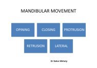
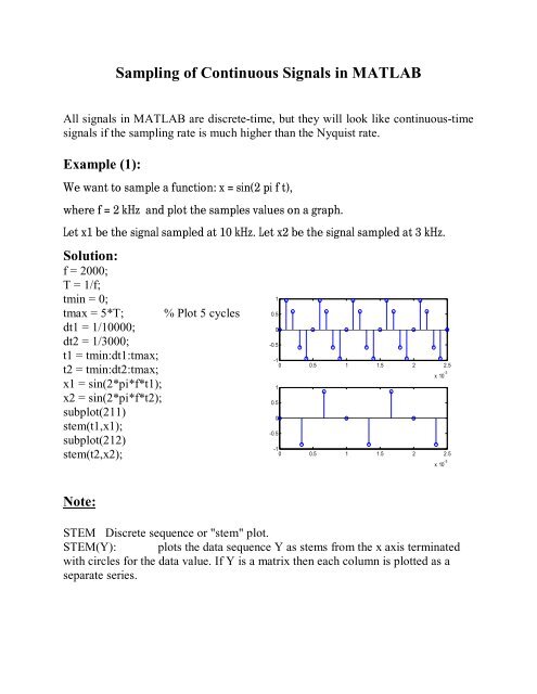
Example (1):
We want to sample a function: x = sin(2 pi f t),
where f = 2 kHz and plot the samples values on a graph.
Let x1 be the signal sampled at 10 kHz. Let x2 be the signal sampled at 3 kHz.
Solution:
f = 2000;
T = 1/f;
tmin = 0;
tmax = 5*T; % Plot 5 cycles
dt1 = 1/10000;
dt2 = 1/3000;
t1 = tmin:dt1:tmax;
t2 = tmin:dt2:tmax;
x1 = sin(2*pi*f*t1);
x2 = sin(2*pi*f*t2);
subplot(211)
stem(t1,x1);
subplot(212)
stem(t2,x2);
1
0.5
0
-0.5
-1
0 0.5 1 1.5 2 2.5
1
0.5
0
-0.5
x 10 -3
-1
0 0.5 1 1.5 2 2.5
x 10 -3
Note:
STEM Discrete sequence or "stem" plot.
STEM(Y): plots the data sequence Y as stems from the x axis terminated
with circles for the data value. If Y is a matrix then each column is plotted as a
separate series.

Example (2):
We want to sample a function: x = sin(2 pi f t),
where f = 2 kHz and display the samples values in a vector.
Let x1 be the signal sampled at 10 kHz. Let x2 be the signal sampled at 3 kHz.
Solution:
% Sample the sinusoid x = sin(2 pi f t), where f = 2 kHz, and
plot the sampled signals over the continuous-time signal.
% Let x1 be the signal sampled at 10 kHz.
% Let x2 be the signal sampled at 3 kHz.
f = 2000;
T = 1/f;
tmin = 0;
tmax = 5*T;
%Sampling rate
dt1 = 1/10000;
dt2 = 1/3000;
for t1 = tmin:dt1:tmax
i=1;
x1(i) = sin(2*pi*f*t1);
i=i+1;
end;
disp(x1);
for t2 = tmin:dt2:tmax;
j=1;
x2(j) = sin(2*pi*f*t2);
j=j+1;
end;
disp(x2);

X1:
Columns 1 through 7
-0.0000 0.9511 0.5878 -0.5878 -0.9511 -0.0000 0.9511
Columns 8 through 14
0.5878 -0.5878 -0.9511 -0.0000 0.9511 0.5878 -0.5878
Columns 15 through 21
-0.9511 -0.0000 0.9511 0.5878 -0.5878 -0.9511 -0.0000
Columns 22 through 26
0.9511 0.5878 -0.5878 -0.9511 -0.0000
X2:
Columns 1 through 7
-0.8660 -0.8660 0.8660 -0.0000 -0.8660 0.8660 -0.0000
Column 8
-0.8660

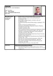
Example (3):
We want to sample a function: x = sin(2 pi f t),
where f = 2 kHz and plot the samples values on a graph containing the original
signal.
Let x1 be the signal sampled at 10 kHz. Let x2 be the signal sampled at 3 kHz.
Solution:
% Sample the sinusoid x = sin(2 pi f t), where f = 2 kHz, and
plot the sampled
% signals over the continuous-time signal.
% Let x1 be the signal sampled at 10 kHz.
% Let x2 be the signal sampled at 3 kHz.
f = 2000;
T = 1/f;
tmin = 0;
tmax = 5*T;
dt = T/100; % take 100 points within each cycle
% for an accurate plot use sufficient points within one cycle
(100,200,500…) Increasing ‘dt’ will decrease the accuracy
t = tmin:dt:tmax;
x = sin(2*pi*f*t);
dt1 = 1/10000;
dt2 = 1/3000;
t1 = tmin:dt1:tmax;
t2 = tmin:dt2:tmax;
x1 = sin(2*pi*f*t1);
x2 = sin(2*pi*f*t2);
subplot(211)
plot(t,x,'r');
hold on
stem(t1,x1); % to display the samples on the original plot
subplot(212)
plot(t,x,'r');
hold on
stem(t2,x2); % to display the samples on the original plot

1
0.5
0
-0.5
-1
0 0.5 1 1.5 2 2.5
x 10 -3
1
0.5
0
-0.5
-1
0 0.5 1 1.5 2 2.5
x 10 -3

MATLAB treatment of audio signals
Recording an audio signal via a microphone:
y = audiorecorder
After you create an audiorecorder object, you can use the methods listed below on
that object.
record(y) Starts recording
record(y,length) Records for length number of seconds.
stop(y) Stops recording
pause(y) Pauses recording
resume(y) Restarts recording from where recording was paused.
play(y) Creates an audioplayer, plays the recorded audio data,
and returns a handle to the created audioplayer.
Reading an audio file .wav
y = wavread(filename) loads a WAVE file specified by filename, returning
the sampled data in y.
[y, Fs, nbits] = wavread(filename) returns the sample rate (Fs) in Hertz and
the number of bits per sample (nbits) used to encode the data in the file.