Evaluation of the Australian Wage Subsidy Special Youth ...
Evaluation of the Australian Wage Subsidy Special Youth ... Evaluation of the Australian Wage Subsidy Special Youth ...
176 5.6.1 Survey design and non-response effects on modelling Mcrae et al. (1985) found that the strong differential response effect for movers and nonmovers affected labour force variables measured in the 1984 survey. They pointed out that models and estimates of such variables might be biased by the non-response, unless the weights were applied. Movers, who had much lower chance of interview, were more likely than non-movers to be older than 20, married and in employment 121 , and had briefer CES registration. The definition of the SYETP treatment group relies on 1984 survey data. The eligibility criteria for SYETP, and the other evidence 122 that they were more likely to be teenagers, hints that SYETP participants would more commonly have been non-movers, and have had a higher response rate. In light of this, the SYETP participation model is first examined, by exploring the effects of the survey weights. The aim is to study the influence of non-response, and so check whether the mobility, age, gender, duration of registration and state of registration were related to the variable of interest here, SYETP participation. 5.6.1.1 Analytical selection Before continuing, the analytical selection from the full data is examined. Recall the limits of the sample: the exclusion from those interviewed in 1984 of those who were over 25 years at the interview date, those in full-time education, or for whom responses were missing in 1984, 1985 or 1986 (Richardson (1998): 5). For the purposes of evaluation analysis of SYETP, only those who were aged less than 25 and not in fulltime education in the 1984 survey interview can be of interest due to the eligibility restrictions for SYETP. These are discarded at different stages of the analysis however. Age was observed in the administrative data, and is accounted for in the non-response weight and so it is 121 Movers were also less likely to be unemployed, but had the same proportions not in the labour force as non-movers. 122 See Chapter 2, for example the results of Hoy and Lampe (1982) covered in Section 2.2.6.2.
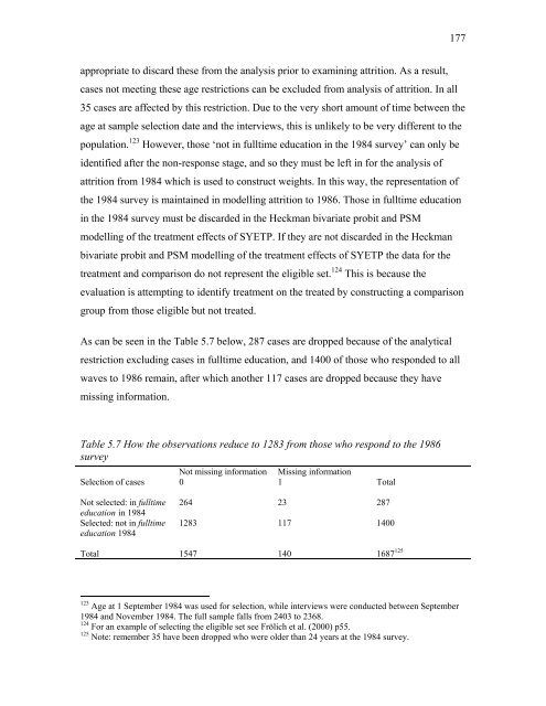
177 appropriate to discard these from the analysis prior to examining attrition. As a result, cases not meeting these age restrictions can be excluded from analysis of attrition. In all 35 cases are affected by this restriction. Due to the very short amount of time between the age at sample selection date and the interviews, this is unlikely to be very different to the population. 123 However, those ‘not in fulltime education in the 1984 survey’ can only be identified after the non-response stage, and so they must be left in for the analysis of attrition from 1984 which is used to construct weights. In this way, the representation of the 1984 survey is maintained in modelling attrition to 1986. Those in fulltime education in the 1984 survey must be discarded in the Heckman bivariate probit and PSM modelling of the treatment effects of SYETP. If they are not discarded in the Heckman bivariate probit and PSM modelling of the treatment effects of SYETP the data for the treatment and comparison do not represent the eligible set. 124 This is because the evaluation is attempting to identify treatment on the treated by constructing a comparison group from those eligible but not treated. As can be seen in the Table 5.7 below, 287 cases are dropped because of the analytical restriction excluding cases in fulltime education, and 1400 of those who responded to all waves to 1986 remain, after which another 117 cases are dropped because they have missing information. Table 5.7 How the observations reduce to 1283 from those who respond to the 1986 survey Not missing information Missing information Selection of cases 0 1 Total Not selected: in fulltime education in 1984 Selected: not in fulltime education 1984 264 23 287 1283 117 1400 Total 1547 140 1687 125 123 Age at 1 September 1984 was used for selection, while interviews were conducted between September 1984 and November 1984. The full sample falls from 2403 to 2368. 124 For an example of selecting the eligible set see Frölich et al. (2000) p55. 125 Note: remember 35 have been dropped who were older than 24 years at the 1984 survey.
- Page 141 and 142: Highest qualification in 1984 (1.56
- Page 143 and 144: 127 4.6 Distribution of the propens
- Page 145 and 146: 129 Figure 4.3 Histograms of estima
- Page 147 and 148: 131 Table 4.5 Summary statistics fo
- Page 149 and 150: 133 Table 4.5, that the variance of
- Page 151 and 152: 135 Table 4.6 Matching results, Sin
- Page 153 and 154: 137 Table 6.3 using Swedish data wi
- Page 155 and 156: 139 matching is the ability to weed
- Page 157 and 158: 141 Table 4.7 Matching results, All
- Page 159 and 160: 143 the unobserved component. If th
- Page 161 and 162: 145 5: Study 3 Attrition and non-re
- Page 163 and 164: 147 occur by design, because the mi
- Page 165 and 166: 149 (1990) extended and improved th
- Page 167 and 168: 151 (10) A* = δ 0 + δ 1 x +δ 2 z
- Page 169 and 170: 153 again from September to Novembe
- Page 171 and 172: 155 5.5.2 Univariate examination of
- Page 173 and 174: 157 lower, the job lengths are only
- Page 175 and 176: 159 Work limited by health 1984 0.1
- Page 177 and 178: 161 The characteristics of the SYET
- Page 179 and 180: 163 para-professional Mother not em
- Page 181 and 182: 165 comparison group where the shar
- Page 183 and 184: 167 5.5.4 Attrition: natural attrit
- Page 185 and 186: 169 both sources that impose change
- Page 187 and 188: 171 para-professional Father not em
- Page 189 and 190: 173 work in later sections, this su
- Page 191: 175 Table 5.6: Effect of selection/
- Page 195 and 196: 179 Australia/Tasmania. Amongst tho
- Page 197 and 198: 181 Table 5.5a Summary statistics b
- Page 199 and 200: 183 5.6.1.2 Effects of the non-resp
- Page 201 and 202: 185 3 years + -0.35 -0.47 -0.34 -0.
- Page 203 and 204: 187 5.7 Multivariate analysis of ef
- Page 205 and 206: 189 proportion of time spent unempl
- Page 207 and 208: 191 post-school qualification, and
- Page 209 and 210: 193 Generally, those variables foun
- Page 211 and 212: 195 longj0 Longest job by 1984 < 1
- Page 213 and 214: 197 adopted in order to maintain co
- Page 215 and 216: 199 6: Study 4 Weighting to counter
- Page 217 and 218: 201 Table 6.1, part A Employment eq
- Page 219 and 220: 203 Methodist 0.133 0.261 (0.77) (1
- Page 221 and 222: 205 CEP referrals 1984 0.143* 0.128
- Page 223 and 224: 207 6.2 Results of weighting the PS
- Page 225 and 226: 209 The distribution of the propens
- Page 227 and 228: 211 Table 6.3 Weighted probit used
- Page 229 and 230: 213 (0.76) Tradesperson mtrad 0.20
- Page 231 and 232: 215 Table 6.5 Summary statistics fo
- Page 233 and 234: 217 Table 6.7 Matching results, sin
- Page 235 and 236: 219 6.3 Discussion The comparison o
- Page 237 and 238: 221 the selection into SYETP and th
- Page 239 and 240: 223 Heteroskedasticity is a violati
- Page 241 and 242: 225 Table 7.1, Part A Employment eq
177<br />
appropriate to discard <strong>the</strong>se from <strong>the</strong> analysis prior to examining attrition. As a result,<br />
cases not meeting <strong>the</strong>se age restrictions can be excluded from analysis <strong>of</strong> attrition. In all<br />
35 cases are affected by this restriction. Due to <strong>the</strong> very short amount <strong>of</strong> time between <strong>the</strong><br />
age at sample selection date and <strong>the</strong> interviews, this is unlikely to be very different to <strong>the</strong><br />
population. 123 However, those ‘not in fulltime education in <strong>the</strong> 1984 survey’ can only be<br />
identified after <strong>the</strong> non-response stage, and so <strong>the</strong>y must be left in for <strong>the</strong> analysis <strong>of</strong><br />
attrition from 1984 which is used to construct weights. In this way, <strong>the</strong> representation <strong>of</strong><br />
<strong>the</strong> 1984 survey is maintained in modelling attrition to 1986. Those in fulltime education<br />
in <strong>the</strong> 1984 survey must be discarded in <strong>the</strong> Heckman bivariate probit and PSM<br />
modelling <strong>of</strong> <strong>the</strong> treatment effects <strong>of</strong> SYETP. If <strong>the</strong>y are not discarded in <strong>the</strong> Heckman<br />
bivariate probit and PSM modelling <strong>of</strong> <strong>the</strong> treatment effects <strong>of</strong> SYETP <strong>the</strong> data for <strong>the</strong><br />
treatment and comparison do not represent <strong>the</strong> eligible set. 124 This is because <strong>the</strong><br />
evaluation is attempting to identify treatment on <strong>the</strong> treated by constructing a comparison<br />
group from those eligible but not treated.<br />
As can be seen in <strong>the</strong> Table 5.7 below, 287 cases are dropped because <strong>of</strong> <strong>the</strong> analytical<br />
restriction excluding cases in fulltime education, and 1400 <strong>of</strong> those who responded to all<br />
waves to 1986 remain, after which ano<strong>the</strong>r 117 cases are dropped because <strong>the</strong>y have<br />
missing information.<br />
Table 5.7 How <strong>the</strong> observations reduce to 1283 from those who respond to <strong>the</strong> 1986<br />
survey<br />
Not missing information Missing information<br />
Selection <strong>of</strong> cases 0 1 Total<br />
Not selected: in fulltime<br />
education in 1984<br />
Selected: not in fulltime<br />
education 1984<br />
264 23 287<br />
1283 117 1400<br />
Total 1547 140 1687 125<br />
123 Age at 1 September 1984 was used for selection, while interviews were conducted between September<br />
1984 and November 1984. The full sample falls from 2403 to 2368.<br />
124 For an example <strong>of</strong> selecting <strong>the</strong> eligible set see Frölich et al. (2000) p55.<br />
125 Note: remember 35 have been dropped who were older than 24 years at <strong>the</strong> 1984 survey.


