A Transient Stability Constrained Optimal Power Flow

Bulk Power System Dynamics and Control IV – Restructuring, August 24-28, Santorini, Greece
A Transient Stability Constrained Optimal Power Flow
Deqiang Gan (M) Robert J. Thomas (F) Ray D. Zimmerman (M)
deqiang@ee.cornell.edu rjt1@cornell.edu rz10@cornell.edu
School of Electrical Engineering
Cornell University
Ithaca, NY 14853
Abstract
Stability is an important constraint in power system
operation. Often trial and error heuristics are used that can
be costly and imprecise. A new methodology that eliminates
the need for repeated simulation to determine a transiently
secure operating point is presented. The methodology
involves a stability constrained Optimal Power Flow (OPF).
The theoretical development is straightforward: swing
equations are converted to numerically equivalent algebraic
equations and then integrated into a standard OPF
formulation. In this way standard nonlinear programming
techniques can be applied to the problem.
Introduction
The cost of losing synchronous operation through a
transient instability is extremely high in modern power
systems. Consequently, utility engineers often perform a
large number of stability studies in order to avoid the
problem. Mathematically, the transient stability problem
is described by solutions of a set of differential-algebraic
equations [1,2,3]. The simplest form of the equations are
the so-called swing equations. The current industry
standard is to solve these equations via step-by-step
integration (SBSI) methods. Since different operating
points of a power system have different stability
characteristics, transient stability can be maintained by
searching for one that respects appropriate stability
limits. Such a search using conventional methods has to
be done by trial-and-error incorporating heuristics based
on engineering experience and judgement. Recently,
significant improvements in computer technology have
encouraged the successful implementation of on-line
dynamic security assessment programs [4,5,6]. While
these new programs greatly improve the ability to
monitor system stability, they also reveal that trial-anderror
methods are not suitable for automated
computation.
The disadvantage of SBSI methods has been recognized
since the early stages of computer application in power
systems. This encouraged extensive investigations into
energy function methods [8,9,10,11]. These methods
have their roots in Lyapunov stability theory and they
provide a quantitative stability margin based on an
assessment of the change in direction of the operating
point [12,13,14]. Possibly for the same reason, research
on pattern recognition and its variant, artificial neural
networks, has also been rather active in the past two
decades. Although these methods do not contain an
explicit stability margin, they do provide for a simple
mapping between controllable generation dispatch and
indices such as an energy margin, rotor angles, etc. The
simple mapping information can in turn be used in a
preventive control formulation [15]. Other attempts to
solve this preventive control problem can be found in, for
example, references [4,16,17,18].
The unique feature of an OPF is that certain costs can be
minimized while functional constraints such as line-flow
and voltage limits are respected. Significant progress has
been made in this area in recent years [19,20,21]. Given
state-of-the-art OPF software, power engineers can
perform studies for large systems with n-1 steady-state
constraints in a reasonable amount of time. It is relatively
straightforward to include n-1 contingency constraints
since these constraints can be modeled via algebraic
equations or inequalities. It is, however, an open question
as to how to include stability constraints since stability is
a dynamic concept and differential equations are
involved. Recently, OPF practitioners began to discuss
the possibility of including stability constraints in
standard OPF formulations [19,21,22]. A few attempts
based on either energy function methods or pattern
recognition techniques have been pursued [12,13,14,15].
The importance of maintaining stability in power systems
operation however calls for fundamentally strict, precise,
yet flexible methodologies.
1

It is also worth mentioning that the emergence of
competitive power markets also creates the need for a
stability-constrained OPF because the traditional trialand-error
method could produce a discrimination among
market players in stressed power systems [23]. As
reported in [24], “the past practice of maintaining
reliability by following operating guidelines based on offline
stability studies is not satisfactory in a deregulated
environment”.
In this paper, we develop a method for handling transient
stability constraints. We demonstrate our idea by
applying it to a stability-constrained OPF problem. The
methodology is built upon a state-of-the-art OPF and
SBSI techniques. By converting the differential equations
into numerically equivalent algebraic equations, standard
nonlinear programming techniques can be applied to the
problem. We demonstrate via simulation results that
stability constraints such as rotor angle limits and/or tieline
stability limits can be conveniently controlled in the
same way thermal limits are controlled in the context of
an OPF solution.
A Stability-Constrained Optimal Power
Flow Formulation
A standard OPF problem can be formulated as follows
[19]:
Min f ( P g
) (1)
S.T. P − P − P( V , θ ) = 0 (2)
g
L
Qg
− QL
− Q( V, θ ) = 0
(3)
S ( V ,θ ) − S M ≤ 0
(4)
m
M
V ≤ V ≤ V
(5)
m
M
P ≤ P ≤ P
(6)
g
g
g
Qg m ≤ Q g ≤ Qg M
(7)
Where f ( ⋅ ) is a cost function; (2) and (3) are the active
and reactive power flow equations, respectively; P g is
the vector of generator active power output with upper
bound P g M and lower bound P g m ; Q g is the vector of
reactive power output with upper bound Q g M
and lower
bound Q g m ; P L and Q L are vectors of real and reactive
power demand; P( V,θ ) and Q( V,θ ) are vectors of real
and imaginary network injections, respectively; S( V,θ)
is a vector of apparent power across the transmission
lines and S M contains the thermal limits for those lines;
V and θ are vectors of bus voltage magnitudes and
angles with lower and upper limits V m and V M ,
respectively. Note that P , Q , V , and θ are the free
variables in the problem.
g
Now, assume that the dynamics are governed by the socalled
classical model in which the synchronous machine
is characterized by a constant voltage E behind a
transient reactance X d
′ . For the sake of illustration the
load is modeled by constant impedance. Note that more
complicated models could be used without loss of
generality. We have the following “swing” equation [1]:
dδi
= ωi
dt
dδ
dt
i
⎡G
⎢
⎣B
πf
0
⎡
H P 1
= ⎢ gi
−
2 i ⎣ X′
di
( , , , , δ , ω )
= D P E W W
i gi i xi yi i i
− B⎤
W
G
⎥
⎦
⋅ ⎡ ⎣ ⎢ W
x
y
⎤ I
⎥ = ⎡ ⎢
⎦ ⎣⎢
I
x
y
g
⎤
( EiWxi sinδi − E
iWyi cosδi)
⎥
⎤
⎥
⎦⎥
⎦
(8)
(9)
(10)
Where G and B contain the real and reactive part of the
bus admittance matrix, respectively; W x
and W y
are
vectors containing the real and imaginary part of the
network (bus) voltages; f 0
is the nominal system
frequency; H i
is the inertia of ith generator; ω i
and δ i
are the rotor speed and angle of ith generator. The ith
entry of I x and I y
is given by:
I
I
xi
xi
Ei
sinδ i E
= , I
i cosδ
yi
= −
X ′
X ′
d
d
i
(generator buses)
= 0, I = 0
(non-generator buses)
yi
We require that a solution of the stability-constrained
OPF respect the following constraint for each i:
ng
∑
k=
1
ng
δ = δ − ≤ 100 o (11)
i
i
∑
k=
1
H δ
k
H
k
k
2

Where ng is the number of generators and δ
i
is the rotor
angle with respect to a center of inertia reference frame.
We use rotor angle to indicate whether or not the system
is stable. Note that other constraints such as voltage dip
can also be included here.
A solution to a stability-constrained OPF would be a set
of generator set-points that satisfy equations (1)-(11) for
a set of credible contingencies. Unfortunately, this hard
nonlinear programming problem contains both algebraic
and differential equation constraints. Existing
optimization methods cannot deal with this kind of
problem directly. In the next section, we propose a
method to attack the problem.
Outline of the Idea
As mentioned in preceding text, it is relatively
straightforward to include n-1 contingency constraints
into OPF since these constraints can be modeled via
algebraic equations or inequalities. It is, however, an
open question about how to include stability constraints.
Obviously the key to solving the problem is in handling
the differential equations. Here we convert the
differential-algebraic equations to numerically equivalent
algebraic equations using trapezoidal rule. This yields:
( )
( D )
δ
i n + 1
δi h
ωi + 1
− − + ωi 2
= 0 (12)
ω i n + 1
ωi h D
n + 1
− − + n
2
= 0 (13)
GV + 1
− BV + 1
− I
+ 1
= 0 (14)
x n y n x n
BV + 1
GV + 1
+ − I
+ 1
= 0 (15)
x n y n y n
( n = 12 , ,..., nend; i = 1, 2,...,
ng)
where h is the integration step length, n is the
integration step counter, and nend is the number of
integration steps [28]. The stability constraints can thus
be expressed as follows:
δ
n
i
ng
∑ Hkδ
k=
1
−
ng
∑ H
k=
1
k
n
k
≤ 100 o (16)
( n = 12 , ,..., nend; i = 1, 2,...,
ng)
Note that we still have to set up the equations for
computing initial values of rotor angle and the equations
for computing parameters of the swing equations. It is
straightforward to show that:
ω i
1
E V
= 0
( θ )
cos( δ θ )
1
sin δ − + P X ′ = 0
i i i i gi di
2 1
i i i i i di gi
0
E − E V − − X ′ Q =
( i = 12 , ,..., ng)
G
B
P
Li
load, i =
2
Vi
load i
(17)
(18)
(19)
(20)
QLi
,
= −
V 2
i
(21)
( i = 1, 2,...,
nb)
Where G load , i and B load , i represent the real and imaginary
part of load impedance, and nb is the number of buses. In
summary, we obtain the following algebraic nonlinear
program (NP) problem:
Min f ( P g
) (22)
S.T. (2) – (7)
(12) – (22)
This standard nonlinear programming problem can be
solved using existing numerical methods. Indeed, the
idea described in this section is surprisingly simple. In
subsequent sections, we will develop a linear
programming (LP) based computational procedure to
solve this algebraic NP problem.
Computational Issues
In this section, we outline the overall procedure of our
method and discuss computational complexities
associated with stability constrained OPF problem.
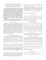
A. An Algorithm
A model algorithm that has been tested on small power
systems is outlined in Fig. 1. We constructed the model
algorithms from direct extension of the successive linear
programming method with constraint relaxation [22].
In what follows we explain the procedure described in
Fig. 1. Since individual stability constraints are typically
not binding, it is only prudent to begin by solving a
standard OPF to start and to check to see if the solution of
3

the standard OPF respects stability constraints. If the
solution does, then this solution is also the final solution
of stability constrained OPF. If the solution does not
respect stability constraints, then a complete stability
constrained OPF must be solved.
Run standard OPF; Run SBSI
steady-state security constrained OPF and dynamicsecurity
constrained OPF. As an example assume
− There 10 contingency constraint equations
− The integration step size is 0.1 second
− The integration period is 2 second
− There are 2 network switches (the point in time
where the fault is applied and cleared)
Are stability constraints violated?
Yes
Solve load flow; execute SBSI
Linearize OPF constraints (2) - (7);
Linearize stability constraints (11) - (21)
Linearize objective function (1)
No
Stop
Note that each integration step imposes one set of
constraints (equations 12-16), so each contingency
imposes a set of 22 constraints (2/0.1 + 2 constraints).
Thus for this stability-constrained OPF problem, 220
constraints need to be appended to standard OPF. For
steady-state security constrained OPF, 10 constraints
would need to be appended to the standard OPF. This
analysis is however overly simplistic for the following
reasons:
Solve the LP problem, update solution
No
Are KT condition satisfied?
Yes
Stop
Fig 1: A procedure for the stability constrained OPF
The KT or Kuhn-Tucker condition alluded to in Fig. 1 is
the optimality condition for the algebraic NP problem.
Inside the main loop, load flow and swing equations are
solved simultaneously. Based on our computational
experience, this seems to be overly cautious. So in our
prototype code, we solve load flow and swing equations
sequentially. Our experience also indicates that the
integration format used in SBSI and that in the algebraic
NP problem should be consistent. Otherwise, the
algorithm may not converge.
Linearizing the objective function and constraints is
trivial. The only thing we would point out is that the
number of stability constraints is very large.
First, for many occasions one is only interested in
transient stability constrained problems in which only one
contingency is involved at a time.
Second, we notice that the number of binding constraints
for dynamic security is typically smaller than that for
steady-state security. In perhaps any power system, the
number of binding stability constraints is normally very
small, say in the order of 5 or less.
Third, for most stability studies, we can apply the
constraint relaxation technique explained below. Suppose
the maximum rotor angle at each integration step, that is
max( δ , i 1,..., ng)
, reaches its maximum point at 0.8
i =
second, then the constraints associated with those
integration steps after, say, 1.0 second can be excluded
from the LP problem (see Fig. 2).
Rotor Angle
100 degrees
B. Computational Complexity
The algebraic NP problem (22) contains a very large
number of constraints. At this point, we are not able to
validate whether or not the LP-based method is efficient
for this problem. Rather, we offer some observations that
could lead to a practical solution to this problem. We
start our discussion by making a comparison between
0.8 Integration Time
Fig. 2. Constraint Relaxation for the Stability
Constrained OPF
4

The above technique, which is conceptually different
from that described in [22], can reduce the size of the LP
problem significantly (note that a full SBSI should
always be performed to make sure that no stability limit
is violated).
An Extension
The integration-based method described in the preceding
sections also offers the basis of an analytical tool for
other stability-related problems. We give some examples
in this section.
Similar to standard OPF or steady-state security
constrained OPF, the objective function of the stability
constrained OPF can be defined as operating cost,
transmission loss, as well as special objectives like the
one given below:
0
∑ 2
i
Min ( P gi
− Pgi)
S.T. (2) – (7)
(11) – (20)
Where
P g
0
represents the desired operating point
(typically the previous one). The objective of this OPF is
to find a secure operating point that is close to the desired
operating point. Such a problem is known as preventive
control or generation rescheduling.
Another example is to estimate the loadability of power
systems subject to stability constraint [25]. The objective
function and load flow constraints in this problem should
be defined as:
Min λ
S.T.
P −λP − P( V , θ) = 0
g
L
Q − λQ − Q( V, θ) = 0
g
L
(4) – (7), (11) – (20)
Where scalar λ denotes a parameter associated with load
increases.
Note that once the TTC is obtained, it is trivial to
compute Available Transfer Capability (ATC) [24]. The
interface flow can be either of the point-to-point or the
area-to-area type.
We would also like to mention that, the method could be
modified to compute Critical Clearing Time (CCT), a
measure of stability margin, for simple contingencies.
The objective function in this case becomes:
Max CCT
More sophisticated implementation has to be formulated
to accommodate CCT computation.
One of the advantages of our method is that it has less
limitation on component modeling. Load can be
expressed as any combination of constant impedance,
constant current, and constant power. Generators can be
modeled with a single-axis model, a two-axis model, or
even a more detailed model [1]. Interesting network
changes such as three-phase-ground faults or the removal
of transmission lines can be modeled in a straightforward
way.
Numerical Examples
The integration-based method was implemented using the
MATPOWER package [26], a MATLAB-based power
system analysis toolbox that is freely available for
download from the site at
http://www.pserc.cornell.edu/matpower/. The prototype
code has been tested on the WSCC 3-machine 9-bus
system and the system New England 10-machine 39-bus
System. The results of New England system are presented
here.
The operating point is given by a standard OPF. A threephase-to-ground
fault is applied to bus 29, the fault is
cleared 0.1 second later coupled with the removal of line
29-28. The integration step size is set to 0.1 seconds and
the integration is executed for 1.5 seconds. We note that
the operating point did not respect the stability constraint
(the relative rotor angle of generator at bus 29 is about
700 degrees at time 1.5 second (See Fig. 3).
Now, the Total Transfer Capability (TTC) or stability
limit of a tie line can be computed by solving:
Max Interface Flow
S.T. (2) – (7)
(11) – (20)
5

800
700
600
500
400
300
200
100
0
0
0.2
0.4
0.6
0.8
OPF
Solution
SOPF
Solution
swing information. We demonstrated that, using this
general methodology, for the first time the stability limits
of power systems can be precisely and automatically
estimated. We are hoping that the methodology can be
developed into a practical tool but this requires that it be
efficiently implemented.
Acknowlegdement
1
1.2
1.4
Fig 3: Maximum Angle (at each integration step)
The stability constrained OPF program was then run
providing an operating point that respects stability
constraints, as illustrated in Fig 3. The operating cost of
the system was slightly increased. The iteration process
in the stability constrained OPF is illustrated in Fig. 4.
800
700
600
500
400
300
200
100
0
1
3
5
Conclusions
Integration Time
7
9
11
13
15
Iteration Counter
Fig 4. Iteration Process of Stability Constrained
OPF
Maximu
m Angle
Cost
In the recent past tremendous effort has been spent on
system stability issues. The objectives are to monitor and
ultimately control the stability during power system
operation. While the technology for stability simulation is
rather stable now, little analytical development has been
done for computing stability limits precisely. This is
perhaps because computing the stability limits precisely
has been thought to be impossible [27].
There is, however, an increasing need for solutions for
this challenging problem. In this paper, we have
developed a basis for one approach to this problem. The
method naturally inherits the advantages of SBSI-based
methods such as, it has little limitations on component
modeling, it is robust, and it provides all relevant system
We would like to thank Z. Yan and C. Murillo-Sanchez
for their valuable help during the course of the study
reported in the paper.
References
1. P.W. Sauer, M.A. Pai, Power System Dynamics and
Stability, Prentice-Hall, Upper Saddle River, New Jersey, 1998
2. P. Kundur, Power System Stability and Control, McGraw-
Hill, 1994
3. B. Stott, “Power System Dynamic Response Calculations”,
Proceedings of the IEEE, vol. 67, no. 2, 1979, pp 219-241
4. E. Vaahedi, Y. Mansour, et al, “A General Purpose
Method for On-line Dynamic Security Assessment”, IEEE
Trans. on Power Systems, vol. 13, no. 1, 1998, pp. 243-249
5. K.W. Chan, R.W. Dunn, et al., “On-line Dynamic-security
Contingency Screening and Ranking”, IEE Proceedings-
Generation Transmission and Distribution, vol. 144, no. 2,
1997, pp. 132-138
6. K. Demaree, T. Athay, et al., “An On-line Dynamic
Security Analysis System Implementation”, IEEE Trans. on
Power Systems, vol. 9, no. 4, 1994, pp 1716-1722
7. C. Pottle, R.J. Thomas, et al., “Rapid Analysis of
Transient Stability: Hardware Solutions”, in Rapid Analysis of
Transient Stability (a Tutorial), IEEE Publication No.
87 TH 0169-3-PWR, 1987
8. H.D. Chiang, “Direct Stability Analysis of Electric Power
Systems Using Energy Functions: Theory, Application, and
Perspective”, Proceedings of the IEEE, vol. 83, no. 11, Nov.
1995, pp 1497-1529
9. M. Pavella, P.G. Murthy, Transient Stability of Power
Systems: Theory and Practice, John Wiley & Sons, Inc., New
York, 1994
10. A.A. Fouad, V. Vittal, Power System Transient Stability
Analysis Using the Transient Energy Function Method,
Prentice-Hall, Englewood Cliffs, 1991
11. M.A. Pai, Energy Function Analysis for Power System
Stability, Kluwer Academic Publishers, 1989
12. A.A. Fouad, J. Tong, “Stability Constrained Optimal
Rescheduling of Generation”, IEEE Trans. On Power Systems,
vol. 8, no. 1, 1993, pp. 105-112
13. J. Sterling, M.A. Pai, et al., “A Method of Secure and
Optimal Operation of a Power System for Dynamic
Contingencies”, Electric Machine and Power Systems, 19-1991,
pp. 639-655
6

14. K.S. Chandrashekhar, D.J. Hill, “Dynamic Security
Dispatch: Basic Formulation”, IEEE Trans. On Power
Apparatus and Systems, vol. 102, no. 7, July 1983, pp 2145-
2154.
15. V. Miranda, J.N. Fidalgo, et al., “Real Time Preventive
Actions for Transient Stability Enhancement with a Hybrid
Neural-optimization Approach”, IEEE Trans. on Power System,
vol. 10, no. 2, 1995, pp. 1029-1035
16. W. Li, A. Bose, “A Coherency Based Rescheduling
Method for Dynamic Security”, Proceedings of PICA, 1997, pp.
254-259
17. D. Gan, Z. Qu, et al., “Methodology and Computer
Package for Generation Rescheduling”, IEE Proceedings-
Generation Transmission and Distribution, vol. 144, no. 3,
May 1997, pp. 301-307
18. R.J. Kaye, F.F. Wu, “Dynamic Security Regions of Power
Systems”, IEEE Trans. On Circuits and Systems, vol. 29, Sept.
1982
19. J. Carpentier, “Towards a Secure and Optimal Automatic
Operation of Power Systems”, IEEE PICA Conference
Proceedings, Montreal, Canada, 1987, pp. 2-37
20. B. Stott, O. Alsac, et al., “Security Analysis and
Optimization”, Proceedings of IEEE, vol. 75, no. 12, 1987, pp.
1623-1644
21. J.A. Momoh, R.J. Koessler, et al., “Challenges to Optimal
Power Flow”, IEEE Trans on Power Systems, vol. 12, no. 1,
1997, pp. 444-455
22. O. Alsac, J. Bright, et al., “Further Developments in LPbased
Optimal Power Flow”, IEEE Trans. On Power Systems,
vol. 5, no. 3, 1990, pp. 697-711
23. R.J. Thomas, R.D. Zimmerman, et al., “An Internet-Based
Platform for Testing Generation Scheduling Auctions”, Hawaii
International Conference on System Sciences, Hawaii, January
1998
24. S.C. Savulescu, L.G. Leffler, “Computation of Parallel
Flows and the Total and Available Transfer Capability”, 1997
PICA Tutorial.
25. D. Gan, Z. Qu, et al., “Loadability of Generation-
Transmission Systems with Unified Steady-state and Dynamic
Security Constraints”, 14th IEEE/PES Transmission and
Distribution Conference and Exposition, Los Angles,
California, September, 1996, pp. 537-542
26. R. Zimmerman, D. Gan, “MATPOWER: A MATLAB
Power System Simulation Package”,
http://www.pserc.cornell.edu/matpower/
27. M. Ilic, F. Galiana, et al., “Transmission Capacity in
Power Networks”, International Journal of Electrical Power &
Energy Systems, vol. 20, no. 2, 1998, pp. 99-110.
28. F. Alvarado, IEEE Transactions on Power Apparatus &
Systems,1979
7