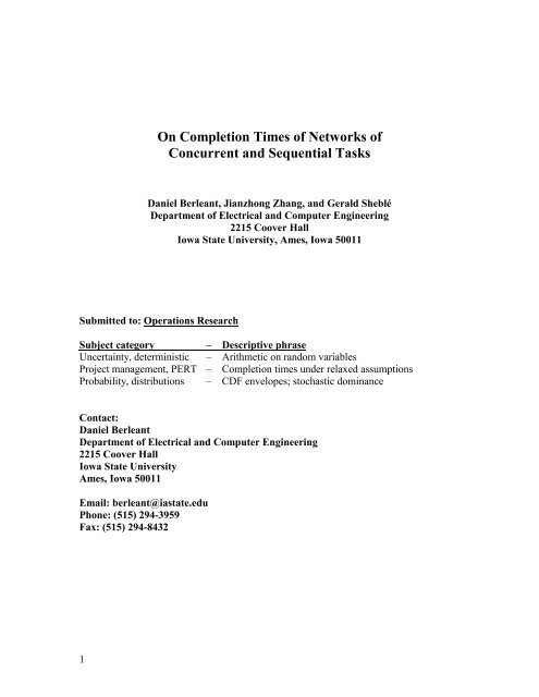
On Completion Times of Networks of Concurrent and Sequential Tasks

On Completion Times of Networks of
Concurrent and Sequential Tasks
Daniel Berleant, Jianzhong Zhang, and Gerald Sheblé
Department of Electrical and Computer Engineering
2215 Coover Hall
Iowa State University, Ames, Iowa 50011
Submitted to: Operations Research
Subject category – Descriptive phrase
Uncertainty, deterministic – Arithmetic on random variables
Project management, PERT – Completion times under relaxed assumptions
Probability, distributions – CDF envelopes; stochastic dominance
Contact:
Daniel Berleant
Department of Electrical and Computer Engineering
2215 Coover Hall
Iowa State University
Ames, Iowa 50011
Email: berleant@iastate.edu
Phone: (515) 294-3959
Fax: (515) 294-8432
1

On Completion Times of Networks of
Concurrent and Sequential Tasks
Daniel Berleant, Jianzhong Zhang, and Gerald Sheblé
Iowa State University, Ames, Iowa 50011
Abstract
The problem of determining the time to complete multiple tasks that may proceed concurrently,
sequentially, or both is considered. In the solution offered, each individual task completion time
may be described with a number, interval, or distribution function. In the case of distribution
functions, two task completion times might be independent random variables, as when the tasks
are performed in different environments and proceed independently. Alternatively, completion
times might be positively correlated, as when both depend on the quality of management and
proceed within the same managerial environment, or they could be negatively correlated, as when
resource sharing means that faster completion of one implies slower completion of the other.
Finally, various factors might interact to make completion times dependent in a way that is
difficult to characterize accurately. The solution offered avoids assuming that individual task
completion times are independent or have any other dependency relationship. One application of
the results is in project management, as in the context of PERT (Program Evaluation and Review
Technique) diagrams.
2

On Completion Times of Networks of
Concurrent and Sequential Tasks
Daniel Berleant, Jianzhong Zhang, and Gerald Sheblé
Iowa State University, Ames, Iowa 50011
berleant@iastate.edu
1 Introduction
Determining the time to complete all tasks in a network of tasks is easy when the time to
complete each individual task in the network has a numerical value, harder when individual
completion times are described using probability distributions, and still more challenging when
these distributions are neither assumed independent nor assumed to have any other dependency
relationship. A method is described here for determining completion times of task networks in the
last case. We begin by describing each task completion time with a probability distribution
function, noting that this includes as a special case a completion time described with a precise
number since a number may be represented as a step distribution function (Figure 1, left). We
later generalize to the case of left and right envelopes enclosing a family of cumulative
distribution functions (CDFs) which, as a special case, allows a completion time to be represented
as an interval describing a range of plausible values with high and low bounds but no information
about the probability distribution within those bounds (Figure 1, right).
1
1
t 1 t→
t lo
t hi
t→
Figure 1. (Left) the numerical value of time t 1 is a special case of a cumulative distribution function
(CDF) which is 0 below t 1 , and 1 at t 1 or above. (Right) an interval [t lo , t hi ] is a special case of a family
of distributions containing any CDF which is 0 below t lo and 1 (at or) above t hi .
3

In real situations, two task completion times might be independent random variables, as
when each is done in a different environment and they proceed independently. Alternatively,
completion times might be highly positively correlated, as could occur if the tasks depend on the
quality of management and proceed within the same managerial environment. As a third
possibility, completion times might be quite negatively correlated, as could occur if the tasks
proceed concurrently with shared personnel or other resources and faster completion of one
entails slower completion of the other. A final and quite likely possibility is that various factors
interact to make completion times dependent in a way that is difficult to characterize accurately.
Therefore in the general case we wish to avoid assuming that individual task completion times are
independent or have any other particular dependency relationship. A solution to this general case
is offered.
The results have application to project management, where task completion time analyses
can be useful as illustrated by the well-known PERT (Program Evaluation and Review
Technique) method.
2 Solution for the case of two concurrent tasks
This section discusses the case of two concurrent tasks. Generalization to larger networks of tasks
is discussed in Section 3.
Consider concurrent tasks X and Y, each beginning when the task environment is in a
start state S and whose joint completion brings about desired finish state F (Figure 2). Let F x be
the CDF of random variable t x , the completion time of task X, and let F y be the CDF of random
variable t y , the completion time of task Y. We begin by reviewing solution strategies when t x and
t y are independent, and then generalize by removing the independence assumption.
One solution strategy is the analytical one. The analytical approach to arithmetic on
random variables is limited in the forms of the distributions it can handle and usually relies on the
assumption of independence (e.g. Springer 1979). The Monte Carlo approach is a numerical
4

strategy that does not produce definite bounds, does not handle cases where one operand is a CDF
and the other an interval except under severe restrictions, does not handle the case of unknown
dependency between random variables, and has other limitations (Ferson 1996). Numerical
convolution (Ingram et. al 1968; Colombo and Jaarsma 1980; Kaplan 1981) is an alternative
numerical strategy that allows arithmetic operations to be applied to random variables with a wide
variety of CDFs, and has been extended to capture discretization error via error bounds that
propagate through the calculations and lead to left and right envelopes around the true solution
(Williamson and Downs 1990; Berleant 1993; Cooper et al. 1996). See Figure 3.
X
S
F
↑
F x
Y
1 1
↑
F y
t→
t→
Figure 2. PERT diagram showing a starting state S, a finish state F, and two tasks X and Y that must
be completed to reach state F. Two different distribution functions F x and F y describe random
variables t x and t y , which represent the completion times of tasks X and Y.
Envelopes consist of non-crossing CDFs that enclose the paths of all CDFs consistent
with the problem. These envelopes are often called probability bounds (Ferson et al. 1998) and,
because they do not cross, the right envelope has first order stochastic dominance over the left
(Levy 1992). Coarse discretizations for random variables t x and t y (e.g. Figure 3) lead to
correspondingly large discretization error and therefore more widely spaced left and right
envelopes. Finer discretizations would result in left and right envelopes that have more and
5

smaller steps and are closer together. The CDF for result t, the time to complete both tasks, must
be some CDF enclosed by the left and right envelopes.
t = max(t x ,t y ), t x and t y independent
[ 2,3]
t ∈
p = 1/8
[ ]
t ∈ 3,4
p = 1/4
[ 4,5]
t ∈
p = 1/8
t
x
[ ]
∈ 1,2
p = ½
[ 2,4]
t ∈
p = 1/8
[ ]
t ∈ 3,4
p = 1/4
[ 4,5]
t ∈
p = 1/8
t
x
[ 2,4]
∈
p = ½
[ 2,3]
t y
∈
p = ¼
t
y
∈ 3,4
p = ½
t
y
[ ]
[ 4,5]
∈
p = ¼
↑
←
t x
t y
Figure 3. Random variable t x is coarsely discretized (bottom row), and similarly for t y (right hand
column). The binary operation appropriate to the task completion problem is max(t x ,t y ) because, for
any samples of t x and t y , both tasks are complete when the one that finishes last is complete. The
distribution of joint completion times is implicit in the set of interior cells (unshaded) of the joint
distribution table, each of which is calculated from its corresponding marginal cells. For example, the
upper left cell contains probability mass 1/8, which is the product of the probabilities of its marginal
cells in the right hand column and bottom row, 1/4 and 1/2 respectively. The product is used because
t x and t y are assumed independent (this assumption will be relaxed later). The upper left cell contains
the interval [2,3] because its marginal cells have task X complete in time [1,2] and Y in time [2,3], so
the time to complete both could potentially be anywhere within that interval. The cumulation over t
of the interior cells is bounded by the left and right envelopes shown, with the separation between the
envelopes due to the undetermined distribution of each cell’s mass across its interval which could, in
extreme cases, be concentrated at the interval low or high bound (Berleant 1993).
Left and right envelopes are each derived from a joint distribution table such as that shown in
Figure 3. The probability mass shown associated with each interior cell of a joint distribution
6

table is the product of the probability masses in its corresponding marginal cells if the operands
are independent, but relaxing the assumption of independence leaves them undetermined.
Therefore when the dependency relationship between the operands is unknown, the process
illustrated in Figure 3 requires significant modification (Berleant and Goodman-Strauss 1998).
Regardless of the dependency relationship between the marginals, the masses of the interior cells
are constrained to some extent by the marginals, which require the masses of all the interior cells
in a row to sum to the mass of the marginal cell at the right of that row, and the masses of the
interior cells in a column to sum to the mass of the corresponding marginal cell at the bottom of
that column. Consequently the summed mass of any particular subset of interior cells will
typically have a range of possible values, and for a properly chosen subset the maximum or
minimum of this range yields a point on the left or right envelope. More specifically, obtaining
the height of the left envelope at time t requires maximizing the collective probability mass of the
interior cells whose intervals have low bounds below (or equal to) t subject to the row and
column constraints, because the mass of each of those cells either may (if the interval’s high
bound is above t) or must (if the interval’s high bound is not above t ) be in the cumulation at t.
The process is analogous for finding the height of the right envelope: minimize the sum of the
probability masses of the interior cells whose intervals have high bounds below or equal to t
(Berleant and Goodman-Strauss 1998). Figure 4 explains the process, which can be done by hand
for a very small table although in the general case linear programming (LP) is more practical. The
left and right envelopes have staircase-like forms. In Figure 4, for example, the heights of the left
and right envelopes at t=3.5 hold for all other values of t between 3 and 4. Because for staircaseshaped
curves the heights for only a limited number of values of t need to be found to fully
characterize the envelopes, the number of LP problems is correspondingly limited. Figure 4 also
shows the full envelopes.
7

Figure 4. An example.
Each interior cell interval in the following joint distribution table has bounds defined by max(t x ,t y )
for its associated (shaded) marginal cell intervals. While interior cell probabilities are constrained by
the marginal cell probabilities, they are not fully determined because no assumptions are made about
the dependency relationship between t x and t y .
t ∈
p 11
[ 2,3]
[ ]
t ∈ 3,4
p 21
t ∈
p 31
[ 4,5]
[ ]
t
x
∈ 1,2
p = ½
t ∈
p 12
[ 2,4]
[ ]
t ∈ 3,4
p 22
t ∈
p 32
[ 4,5]
t x
∈
p = ½
[ 2,4]
t y
∈[ 2,3]
p = ¼
t y
∈[ 3,4]
p = ½
∈[ 4,5]
t y
p = ¼
↑
←
t x
t y
Consider for example the cumulative probability of t at 3.5. Bolded probabilities masses p 11 , p 12 , p 21 ,
and p 22 can contribute to the left envelope of t at 3.5, because the low bounds of the intervals in those
cells are ≤3.5. Therefore those probabilities could all be in the cumulation at t=3.5, and in the
extreme case that p 12 , p 21 , & p 22 happen to be concentrated at the low bounds of their intervals, will
be (and to find points on the envelopes, we are interested in extreme cases). To maximize this
cumulation of p 11 , p 12 , p 21 , and p 22 , their sum must be maximized (at the expense of non-bolded
probabilities p 31 and p 32 ), yielding p 11 +p 12 ,+p 21 +p 22 =3/4 as shown in the following solution:
[ 2,3]
t ∈
p 11 =¼
[ ]
t ∈ 3,4
p 21 =0
[ 4,5]
t ∈
p 31 =¼
[ ]
t
x
∈ 1,2
p = ½
[ 2,4]
t ∈
p 12 =0
[ ]
t ∈ 3,4
p 22 =½
[ 4,5]
t ∈
p 32 =0
t x
∈
p = ½
[ 2,4]
t y
∈[ 2,3]
p = ¼
t y
∈[ 3,4]
p = ½
∈[ 4,5]
t y
p = ¼
↑
←
t x
t y
(continued on next page)
8

(Figure 4 continued)
For the other envelope, the (unary “sum” of) italicized probability mass p 11 is minimized, yielding 0
as shown in the following solution:
[ 2,3]
t ∈
p 11 =0
[ ]
t ∈ 3,4
p 21 =½
[ 4,5]
t ∈
p 31 =0
[ ]
t
x
∈ 1,2
p = ½
[ 2,4]
t ∈
p 12 =¼
[ ]
t ∈ 3,4
p 22 =0
[ 4,5]
t ∈
p 32 =¼
t x
∈
p = ½
[ 2,4]
t y
∈[ 2,3]
p = ¼
t y
∈[ 3,4]
p = ½
∈[ 4,5]
t y
p = ¼
↑
These maximum and minimum cumulations of 3/4 and 0 hold not only for t=3.5 but also for all other
t from 3 to 4, because no interior cell has an interval with an endpoint in that range, as graphed next.
←
t x
t y
Repeating this process for appropriate values of t yields the following full envelopes around
t=max(t x ,t y ).
Although the marginals used here are
the same as in Figure 3, the envelopes
are farther apart because the
dependency between the random
variables is unspecified, so the
inferential power of the independence
assumption is absent. The
discretization, coarse in this example,
also affects the degree of separation of
the envelopes. Finer discretization would yield smaller steps in the envelopes and hence envelopes
that are, on average, closer together.
Figure 4 (end).
9

When linear programming is applied to minimization and maximization problems of this
type the objective function is the sum of the probabilities of the subset of interior cells to be
maximized or minimized, and the constraint set consists of one for each row and one for each
column. A general-purpose linear programming algorithm such as the simplex method can be
used, but a faster choice is the transportation simplex method, which applies to certain problems
such as these containing only row and column constraints.
To apply the transportation simplex method to optimize the distribution of
probability masses across interior cells, the cost coefficients of the cells in the subset
whose probability mass is to be maximized or minimized are set to one, the cost
coefficients of the remaining cells are set to zero, and the allocations of the cells are their
probability masses. In our software implementation, problems involving generating
envelopes from a 16x16 joint distribution table require approximately 14 seconds using
the simplex algorithm but only 1 second using the transportation simplex algorithm, on a
Pentium III PC running Windows NT.
3 Generalizing the solution to networks of concurrent and sequential tasks
Extending the approach from two concurrent tasks to larger networks of tasks requires solving
three problems: (1) determining the completion time of two tasks that run not concurrently but
sequentially, (2) determining the completion time of three or more concurrent tasks, and (3) using
results as inputs to obtain further downstream results. These problems may be solved as follows.
(1) To determine the completion time of two sequential tasks, their individual completion
times are added, because one completes and then the next begins. To add them, the same
procedure that was described earlier for concurrent tasks is applied except that the
intervals in the interior cells of the joint distribution table are obtained by performing
10

t x +t y instead of max(t x ,t y ). Thus for each joint distribution tables in Figure 4, the top left
cell would contain the interval [3,5]=[1,2]+[2,3] instead of [2,3]=max([1,2],[2,3]).
(2) To handle three concurrent tasks, the result for two of them is calculated, and that result
used as the completion time for a composite task that proceeds concurrently with the third
task. In other words, for concurrent tasks X, Y, & Z, we wish to calculate
max(max(x t ,y t ), z t ). This is a case of using intermediate results as inputs, discussed next.
(3) To use a result as an input to another calculation, we must convert a pair of left and right
envelopes, which is what a result looks like, into a set of intervals and associated
probability masses, which is what a marginal in a joint distribution table looks like. To
convert, first note that the envelopes consist of horizontal and vertical line segments. This
allows the space they enclose to be partitioned into a stack of rectangles (Figure 5, top).
Each rectangle defines an interval whose low bound is a value on the horizontal axis at
which there is a vertical segment of the left envelope (forming the left side of the
rectangle), and whose high bound is a value on the horizontal axis at which there is a
vertical segment of the right envelope (forming the right side of the rectangle). The mass
of the interval is the increment in the cumulative probability represented by the (bottomto-top)
height of the rectangle. The result of this partition process is a set of intervals and
their associated probabilities, usable as a marginal in a joint distribution table for another
arithmetic operation (Figure 5, bottom).
4 Using inferences from result envelopes
Consider three types of inference that may be drawn from a pair of left and right envelopes.
1) The probability of finishing all the tasks by some time T 0 is at least P 0 in Figure 6.
Similarly, the probability of not finishing by time T 0 is at least (1-P 1 ).
11

t=max(t z ,t w )
t ∈
p=
[ 2,5]
[ ]
t ∈ 3,5
p=
t ∈
p=
t
z
[ 4,5]
[ ]
∈ 2,5
p = 0.2
t ∈
p=
[ 2,7]
[ ]
t ∈ 3,7
p=
t ∈
p=
t
z
[ 4,7]
[ 2,7]
∈
p = 0.1
t ∈
p=
t ∈
p=
t ∈
p=
t
z
[ 6,7]
[ 6,7]
[ 6,7]
[ ]
∈ 6,7
p = 0.3
t ∈
p=
t ∈
p=
t ∈
p=
t
z
[ 6,9]
[ 6,9]
[ 6,9]
[ ]
∈ 6,9
p = 0.3
[ ]
t ∈ 8,9
p=
[ ]
t ∈ 8,9
p=
[ ]
t ∈ 8,9
p=
t
z
[ ]
∈ 8,9
p = 0.1
t
w
[ ]
∈ 2,3
p = 0.25
t
w
[ ]
∈ 3,4
p = 0.5
t
w
[ ]
∈ 4,5
p = 0.25
↑
←
t z
t w
Figure 5. Staircase shaped envelopes partitioned into a set of intervals and masses (top).
These might represent a random variable t z =max(t x ,t y ), used as a marginal in the last row of
a joint distribution table (bottom), and combined with the concurrent completion time t w of
some other task W. The interior cell probabilities of the table are undetermined since no
dependency relationship was defined between the marginals, and so cannot be given values.
12

Figure 6. Left and right envelopes associate probability intervals with time points. If the
envelopes describe cumulative probability of task completion over time, then the probability
of completion by time T 0 is within the interval [P 0 ,P 1 ], and by time T 1 , [P 2 ,1].
2) Suppose that p(some outcome)∈[P,1]. For example in Figure 6, p(task completion by
time T 1 )∈[P 2 ,1]. The interval [P 2 ,1] is qualitatively different from a point estimate
somewhere between P 2 and 1 that would derive from an analysis that produced a single
distribution function instead of left and right envelopes. This is because, unlike a point
estimate, p∈[P 2 ,1] indicates the plausibility of two distinct scenarios with different
implications, (1) certain completion (within the model limits), and (2) uncertain
completion. Decisions about resource allocation on the overall project or about deadlines
to contract for could depend on which scenario is correct, yet the implied opportunity to
seek further information to enable discriminating, or at least to reduce the second order
uncertainty in completion time would not be available from an analysis that produced a
point probability estimate.
3) Consider the problem of determining the probability that one task will finish later than
another, p(t y >t x ). The probability of one task or path taking longer than another is relevant
in such applications as project management where task networks represent PERT
diagrams describing the prerequisite structure of tasks in a project. A simple example is
13

two tasks that begin at the same time, as in Figure 1. A generalization is two tasks
embedded in a network of tasks, such as in Figure 7 for final tasks CF and EF. In the
generalization the tasks need not start at the same time, and the times at which they
complete depend on both the task itself and any prerequisite tasks in the network. These
prerequisite tasks may form a simple sequence as in the case of task EF with prerequisite
partial path SDE, or contain concurrency as in the case of task CF with prerequisite,
concurrent, partial paths SAC and SBC.
Figure 7. A network of tasks. The times to complete tasks SB and SD are shown as
cumulative distributions. The time to reach state E is the sum of the times to complete SD
and DE, and if the dependency relationship between the completion times for SD and DE are
unknown the sum is a pair of envelopes rather than a single cumulative distribution.
Solving this type of problem requires determining p(t y >t x ), where t x and t y are sample
values of random variables for the time points at which two tasks X and Y, or CF and EF,
etc., complete. To do this, and relate it to standard techniques, we first provide a
continuous solution for the case of independent distributions, then give the discrete form
of the solution, then an intervalized discrete form, and finally remove the independence
assumption.
14

In the case of a continuous solution for independent distributions, if the density
functions of the task completion times are f x
(t)
and f y
(t)
and sample completion times
are t x and t y , then
∞
( f
x
( t0 ) dt .
t= −∞
−∞< t0
< t
(1) p t
y
> t
x
) = f
y
( t)
dt
Intuitively,
f
x
−∞<
t0
< t
( t 0
) dt is the area under f
x
over all times earlier than some given time t,
which is p(t>t x ), or the probability that t is later than the completion time t x of task X. The
probability that the completion time of task Y is within a time period centered at t with
width dt is p(
∈ t ± dt )= f y
( t)
dt.
The probability of both (t>t x ) and t 1
y
∈ t ± dt)
is
t y 2
1
(
2
therefore the product of their individual probabilities,
f
y
( t)
dt f ( t0 ) dt , and
x
−∞<
t0
< t
integrating this expression over all possibilities for t gives equation (1).
∞
(
f
x(
t ) ∆t
for values of t and
0 t= −∞
−∞< t0<
t
Discretizing (1) gives p t > =
y
tx)
f
y
( t)
∆t
t 0 spaced ∆t apart. This can be intervalized, bounding the discretization error and giving
(2)
p(
t
y
) =
p(
Ty
)
p(
T
x
) ,
Tx
p(
T
y
)
> t
x
Ty
Tx , Ty
> Ty
Tx
, Ty
> T
p(
T
x)
x
where the T x and T y are intervals over t x and t y such as might appear in the marginals of a
joint distribution table, p(T x ) and p(T y ) are their associated probability masses, and
T , T , T and Ty
are their low and high bounds.
x
y
x
As an example of equation (2) consider the joint distribution table in Figure 8.
The low bound of p(t y >t x ) is the sum of the probability masses of cells labeled True,
which is 0.789. The high bound is the sum of the masses of cells labeled True or Uncertain,
which is 0.939, yielding p ( t y
t ) ∈[0.789,0.939]
.
> x
15

To remove the independence assumption, the masses of the interior cells are
reapportioned among the interior cells within the limits imposed by the row and column
constraints using linear programming to minimize the summed masses of the cells labeled
True, giving a low bound of 0.61, and then reapportioned again to maximize the summed
masses of the cells labeled True or Uncertain, giving a high bound of 1. The new result,
p ( t y
t ) ∈[0.61,1]
, as expected is wider than the earlier result of
> x
p ( t y
t ) ∈[0.789,0.939]
, which benefited from assuming independence.
> x
t y >t x , t x and t y independent
True
p=.005
True
p=.01
True
p=.02
True
p=.01
True
p=.005
[5,6]
p=.05
True
p=.006
True
p=.012
True
p=.024
True
p=.012
True
p=.006
[6,7]
p=.06
True
p=.008
True
p=.016
True
p=.032
True
p=.016
True
p=.008
[7,8]
p=.08
True
p=.01
True
p=.02
True
p=.04
True
p=.02
True
p=.01
[8,9]
p=.1
True
p=.021
Uncertain
p=.021
True True
p=.042 p=.042
True True
p=.084 p=.084
True True
p=.042 p=.042
True True
p=.021 p=.021
[9,10]
p=.21
[10,11]
p=.21
Uncertain
p=.01
Uncertain
p=.02
True
p=.04
True
p=.02
True
p=.01
[11,12]
p=.1
False
p=.008
Uncertain
p=.016
Uncertain
p=.032
True
p=.016
True
p=.008
[12,13]
p=.08
False
p=.006
False
p=.012
Uncertain
p=.024
Uncertain
p=.012
True
p=.006
[13,14]
p=.06
False
p=.005
False
p=.01
False
p=.02
Uncertain
p=.01
Uncertain
p=.005
[14,15]
p=.05
[10.1,11.1]
p=.1
[11.1,12.1]
p=.2
[12.1,13.1]
p=.4
[13.1,14.1]
p=.2
[14.1,15.1]
p=.1
↑
←
t x
t y
Figure 8. Joint distribution table representing t y >t x , for independent t x and t y . Each interior
cell is labeled True if t y >t x for t y and t x in the intervals of the marginal cells of that interior
cell,, False if instead t y t x for all, some, or none of the interior cell mass).
To restate an example, this process could be used to bound the probability that
the completion time of task X will be later than that of task Y in a PERT diagram
conforming to Figure 1. The process could also be used in a more complex example such
as bounding the probability that task CF will complete later than task EF in Figure 7. The
completion time of each of these tasks will be in the form of envelopes, which when
16

converted to marginals will have overlapping intervals as in Figure 5. However any
overlap is irrelevant to equation (2), which justifies Figure 8. Ultimately such results
could support management decisions about resource allocation intended to optimize the
overall completion time of the entire project.
5 Software
Crystal Ball (www.decisioneering.com) and @risk (www.palisade.com) are well-known
commercial products that rely on Monte Carlo simulation, thereby inheriting the shortcomings of
Monte Carlo simulation noted earlier in Section 2.
RiskCalc (Ferson et al. 1998) is a commercially available package that can do the
operations on random variables used here, although its algorithm (Williamson and Downs, 1990)
is different and more complicated than the one used here, some further details of which have been
described by Berleant and Goodman-Strauss (1998). Our software, Statool, is downloadable from
http://www.public.iastate.edu/~berleant/statool.html. Both systems run under Windows on a PC.
Statool requires Visual Basic to be installed.
6 Conclusion
We have shown how to solve a simply stated problem with significant implications: determining
completion times of networks of tasks in the absence of assumptions about both the forms of
distribution functions and their independence or other dependency relationships. Results are left
and right envelopes bounding the space of plausible CDFs. Completion times of individual tasks
may be expressed as numbers, intervals, distribution functions, or left and right envelopes.
Real problems frequently pose a variety of uncertainties. Therefore methods for obtaining
results with minimal assumptions and while accounting for uncertainty remain an important area
of investigation.
17

7 Acknowledgements
The authors are grateful to Helen Regan, National Center for Ecological Analysis and Synthesis,
University of California, Santa Barbara, for numerous valuable comments.
8 References
BERLEANT, D. 1993. Automatically verified reasoning with both intervals and probability
density functions, Interval Computations (1993 No. 2) 48-70.
BERLEANT, D. AND C. GOODMAN-STRAUSS. 1998. Bounding the results of arithmetic
operations on random variables of unknown dependency using intervals, Reliable
Computing 4 (2) 147-165.
COLOMBO, A.G. AND R.J. JAARSMA. 1980. A powerful numerical method to combine
random variables, IEEE Trans. on Reliability R-29 (2) 126-129.
COOPER, J.A., S. FERSON AND L.R. GINZBURG. 1996. Hybrid processing of stochastic and
subjective uncertainty data, Risk Analysis 16 (6) 785-791.
FERSON, S. 1996. What Monte Carlo methods cannot do, Journal of Human and Ecological
Risk Assessment 2 (4) 990-1007.
FERSON, S., W.T. ROOT, AND R. KUHN. 1998. RAMAS Risk Calc: Risk Assessment with
Uncertain Numbers, Applied Biomathematics, Setauket, NY, www.ramas.com.
INGRAM, G.E., E.L. WELKER, AND C.R. HERRMANN. 1968. Designing for reliability based
on probabilistic modeling using remote access computer systems, in Proc. 7 th Reliability
and Maintainability Conference, American Society of Mechanical Engineers, pp. 492-500.
KAPLAN, S. 1981. On the method of discrete probability distributions in risk and reliability
calculations – application to seismic risk assessment, Risk Analysis 1 (3) 189-196.
18

LEVY, H. 1992. Stochastic dominance and expected utility: survey and analysis, Management
Science 38 (4) 555-593.
SPRINGER, M.D. 1979. The Algebra of Random Variables, John Wiley & Sons, Inc. New York.
WILLIAMSON, R. AND T. DOWNS. 1990. Probabilistic arithmetic I: numerical methods for
calculating convolutions and dependency bounds, International Journal of Approximate
Reasoning 4, 89-158.
19