Generalized Line Outage Distribution Factors - Power Systems ...

2
In terms of (3), the bracketed term in (6) is
with t ( 1 )
( 1 )
l , and so w ( l % 1
)
∆ l % given by (6) simulates the line %l 1
outage impacts.
We proceed with the generalization for multiple-line outages
by next considering the case of the outages of the two
lines %l 1
and %l 2
.We simulate the impacts on , by introducing
ς % l
k
f l k
, taking explicitly into account the inter-
w ( l % 1
) and w ( l % 2
)
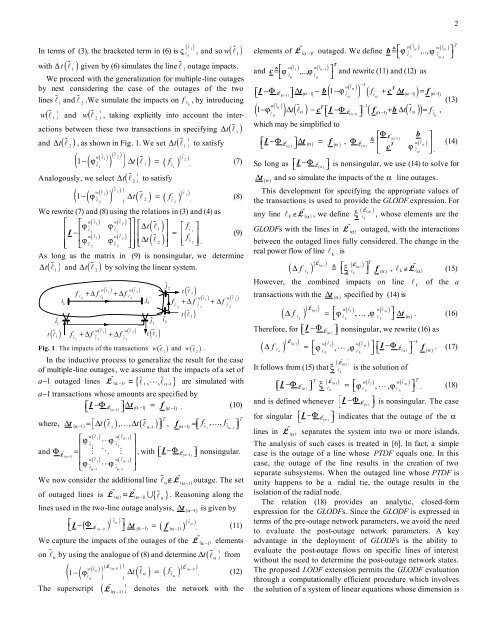
actions between these two transactions in specifying ∆ t( l % 1
)
and ∆ t( l % ) , as shown in Fig. 1. We set ∆ t( l % ) to satisfy
2
( ) ( ) ( ) ( )
w( % )
( ) ( %l
l ) 2
1 l%
2
1− ϕ % ∆ t %l
1
= f
l
% l .
(7)
1 1
Analogously, we select t( )
∆ l % 2
to satisfy
w( % )
( ) ( %l
l ) 1
2 l%
1
1− ϕ % ∆ t %l
2
= f
l
% l .
(8)
( ) ( ) ( ) ( )
2 2
We rewrite (7) and (8) using the relations in (3) and (4) as
⎡ ⎡ w %
( 1) w( 2 )
ϕ
l
l%
ϕ ⎤ ⎤ ⎡ t( 1 ) ⎤ % % ∆ %l ⎡ f %
⎢ ⎢ ⎤
l1 l1
⎥
l 1
I − ⎥ ⎢ ⎥
w( %
1) w( %
2 )
= ⎢
ϕ ϕ t ( 2 )
f
⎥ (9)
⎢ ⎢ l
l
⎥⎥
⎢∆
%l ⎥ ⎢ %l
⎣ 2
⎢ % ⎥⎦
.
⎣ ⎣ l
%
2 l 2 ⎦⎥⎦
⎣ ⎦
As long as the matrix in (9) is nonsingular, we determine
t ∆ t l % by solving the linear system.
∆ ( l % ) and ( )
1
2
Fig. 1. The impacts of the transactions w (% l ) and w (% )
1 l .
2
In the inductive process to generalize the result for the case
of multiple-line outages, we assume that the impacts of a set of
L % α −1 = l % 1, Ll , %
α−1
are simulated with
a−1 outaged lines ( ) { }
a−1 transactions whose amounts are specified by
⎡I − F
( 1) ( α −1 ⎣
∆ α − ) =
L % ⎤ t f
⎦
( α −1)
, (10)
where, ∆ t ( α −1 ) = ⎡∆ (% ) , K,
∆ ( l%
)
T
⎣ t l t ⎤
1
α−1
⎦ , f f , , f
( α 1 %
) ⎣
K
l %
1 lα−1
w( % l1) w( l%
α−1)
ϕ ⎤
% L
l
%
1 l1
⎥
M O M ⎡⎣
I − L%
⎤
α −1 ⎦
w( % l1) w( l%
α−1)
ϕ ⎥
% L
l
%
α−1 lα
−1
1
− =⎡ ⎤⎦
⎡ϕ
⎢
and F L % =
( α−1
) ⎢ ⎥ , with F nonsingular.
( )
⎢
⎣
ϕ
⎦
We now consider the additional line l% α∉L %
( α −1)
outage. The set
of outaged lines is L% ( ) = L% ( ) U{ l%
} . Reasoning along the
α α−1 α
lines used in the two-line outage analysis, ∆t ( α −1)
is given by
(
( )
) ( ) α
⎡
⎤
( ) ( ( ) ) ( ) α
⎣I − % l
l
F
α −1 ⎦ ∆ t α −1 = f
%
L %
α −1 . (11)
We capture the impacts of the outages of the L %( ) elements
on
t (% l 1 )
i
k
w( 1) w( 2)
f +∆ f % l
l
+∆f
%
l lk l
k k
i% j% i%
1
1 2
w( 1) w( 2
f +∆ f % l
l
+∆f
% )
% l1 l% %
1 l1
α −1
%l α
by using the analogue of (8) and determine t( α
)
( )
( ) ( L% )
( %
w %l
α −1 L
( α 1)
)
α
−
1−
ϕ
∆ t %l f
α = %l .
%l
α
α
( ) ( ) ( )
( )
( )
∆ % l from
T
(12)
The superscript L %
( )
denotes the network with the
α −1
j
k
t (% l 1 )
j%
2
t (% l 2 )
w( 1) w( 2
f +∆ f % l
l
+∆f
% )
% l 2 l% %
2 l 2
t (% l 2 )
elements of L %( ) outaged. We define
α −1
w( % l ) w( %
α
lα
)
b @ ⎡ϕ
,.., ϕ ⎤ ⎣ l% %
1 lα
−1
⎦
T
w
and
( l% 1) w( l%
⎡
1)
ϕ ,.., ϕ
α −
c @
⎤ and rewrite (11) and (12) as
% %
⎣ lα
lα
⎦
−1
w( %l α )
T
⎡⎣
I −F
L% ( )
⎤
1 ( 1)
( 1 ) ( f
α α ϕ
− ⎦
∆t − − b − + c ∆ t( α−1)
) = f
l% ( 1)
α l%
α −
α
(13)
w( %l α )
−1
( 1 −ϕ
) ∆t( % T
% lα
) −c ⎡ − ⎤
( )
( ( ) ( ))
1
1 t α f ,
α
⎣
I F %
α−
⎦
f α − + b ∆ l%
=
l
L
% lα
which may be simplified to
⎡ % b ⎤
( α −1)
⎡I −F % ⎤∆ t
( α ) ( α ) = f
⎣ L
⎦
( α )
, % @ F L
F ⎢
w( %
L α ) ⎥
( α )
T
l (14)
⎣
c ϕ %l α ⎦ .
So long as ⎡I −F L%
⎣
⎤
( α ) ⎦ is nonsingular, we use (14) to solve for
∆t and so simulate the impacts of the α line outages.
( α )
This development for specifying the appropriate values of
the transactions is used to provide the GLODF expression. For
any line k ∉ %
( L ( α)
)
l L ( ) , we define ξ %
, whose elements are the
α
GLODFs with the lines in L %
( ) outaged, with the interactions
α
between the outaged lines fully considered. The change in the
real power flow of line l is
k
( f l )
l k
T
( )
∆ @ ⎡ξ
⎤
⎣ ⎦ f
k
( L% ( α ) ) L%
( α )
lk
l ∉ L % (15)
( α )
, k ( α )
However, the combined impacts on line l of the a
k
transactions with the ∆t ( α ) specified by (14) is
( L% ( α ) ) w( l% 1 ) w( l%
α )
( ∆ f ) = ⎡ϕ
, , ϕ ⎤ ∆
k ⎣
K
k k ⎦
t
l l l
( α )
. (16)
Therefore, for ⎡⎣
I −F L%
⎤
( α ) ⎦ nonsingular, we rewrite (16) as
( L%
( ) ) −1
α
w( 1 ) w( α )
( ∆ f ) = ⎡ϕ
l % l%
, , ϕ ⎤ ⎡I
− % ⎤
l k ( α )
k k ⎣ ⎦
f
( α
⎣
L
F L . (17)
l l ⎦
)
( L ( α)
)
It follows from (15) that is the solution of
ξ %
l k
F ( ) ( ) ( )
, (18)
T L% T
( α )
w l% 1
w l%
α
⎡⎣I
− L%
ξ = ⎡
( α )
⎤⎦ ϕ , , ϕ ⎤
l k ⎣ l L
k l k ⎦
and is defined whenever ⎡I −F L%
⎣
⎤
( α ) ⎦ is nonsingular. The case
for singular ⎡I −F L%
⎣
⎤
( α ) ⎦ indicates that the outage of the α
lines in L %
( ) separates the system into two or more islands.
α
The analysis of such cases is treated in [6]. In fact, a simple
case is the outage of a line whose PTDF equals one. In this
case, the outage of the line results in the creation of two
separate subsystems. When the outaged line whose PTDF is
unity happens to be a radial tie, the outage results in the
isolation of the radial node.
The relation (18) provides an analytic, closed-form
expression for the GLODFs. Since the GLODF is expressed in
terms of the pre-outage network parameters, we avoid the need
to evaluate the post-outage network parameters. A key
advantage in the deployment of GLODFs is the ability to
evaluate the post-outage flows on specific lines of interest
without the need to determine the post-outage network states.
The proposed LODF extension permits the GLODF evaluation
through a computationally efficient procedure which involves
the solution of a system of linear equations whose dimension is
T