Generalized Line Outage Distribution Factors - Power Systems ...

1
Abstract— Distribution factors play a key role in many system
security analysis and market applications. The injection shift
factors (ISFs) are the basic factors that serve as building blocks
of the other distribution factors. The line outage distribution
factors (LODFs) may be computed using the ISFs and, in fact,
may be iteratively evaluated when more than one line outage is
considered. The prominent role of cascading outages in recent
black-outs has created a need in security applications for
evaluating LODFs under multiple-line outages. In this letter, we
present an analytic, closed-form expression for and the
computationally efficient evaluation of LODFs under multipleline
outages.
Index Terms—power transfer distribution factors, line outage
distribution factors, multiple-line outages, system security.
I. INTRODUCTION
Distribution factors are linear approximations of the
sensitivities of specific system variables with respect to
changes in nodal injections and withdrawals [1]-[5]. While the
line outage distribution factors (LODFs) are well understood
[1], the evaluation of LODFs under multiple-line outages has
received little attention. Given the usefulness of LODFs in the
study of security with many outaged lines, such as in blackouts
impacting large geographic regions, we focus on the fast
evaluation of LODFs under multiple-line outages – the
generalized LODFs or GLODFs. This letter presents an
analytic, closed-form expression for, and the computationally
efficient evaluation of, GLODFs.
II. BASIC DISTRIBUTION FACTORS
We consider a power system consisting of (N+1) buses and
L lines. We denote by N = { 0,1, K,
N}
the set of buses, with
the bus 0 being the slack bus, and by L = { l ,.., l
1 L } the set of
transmission lines. We associate with each line l L , the
m ∈
ordered pair of nodes (i m , j m ). We us the convention that the
direction of the real power flow f l on the line l is from i
m
m
to
j . m
The ISF
Generalized Line Outage Distribution Factors
Teoman Güler, Student Member, IEEE , and George Gross,
Fellow, IEEE and Minghai Liu, Member, IEEE
i
ψ l k
change in the line
m
of line l is the (approximate) sensitivity of the
k
l real power flow
k
f l with respect to a
k
change in the injection p i at some node i∈N and the
withdrawal of an equal change amount at the slack bus. Under
the lossless conditions and the typical assumptions used in DC
−1
power flow, we construct the ISF matrix Y @ B AB [5], with
Manuscript received June 26, 2006. Research is supported in part by
PSERC. T. Guler and G. Gross are with the Department of Electrical and
Computer Engineering, University of Illinois at Urbana-Champaign,
Urbana, IL 61801 USA (e-mail:tguler@uiuc.edu, gross@uiuc.edu). M. Liu
is with CRAI, Boston, MA 02116 USA (e-mail: mliu@crai.com)
d
L×
L
with B ∈¡ being the branch susceptance matrix,
d
L N
A ∈¡ the reduced incidence matrix and ∈
N × N
B ¡ the
reduced nodal susceptance matrix.
We evaluate the power transfer distribution factors (PTDFs)
by introducing notation for transactions. The impact of a ? t-
MW transaction from node i to node j, denoted by the ordered
w
triplet w@ { i, j, ∆t}
, on f l is ∆ f
k
l , and is determined by
k
w
where the PTDF ϕ l is defined as [5]
For the line
the flow
k
w i j
lk l k lk
∆ f = ϕ ∆t
w w
lk
l ,
k
ϕ @ ψ −ψ
. (2)
l outage, we evaluate the impact
m
f l on line l using the LODF
k
k
( m )
ς l
k
∆ f
( l )
m
l on
k
l which specifies
the fraction of the pre-outage real power flow on the line
redistributed to the line l [5] and is given by:
k
ς
( l m )
l
k
( lm) w( lm
)
l ϕ
k
lk
=
w( l m )
l 1−
ϕ l
m
( )
m
l
m
∆ f
@ , l ≠ l . (3)
k m
f
Here, w( l ) = { i , j , ∆t}
denotes the transaction between the
m m m
w ( l )
( )
ς l
m
m
terminal nodes of l . As long as ϕ ≠ 1
k
l ,
m
l is defined.
k
The line l outage results in a topology change and
m
necessitates reevaluation of the post-outage network PTDFs.
We use the notation ( τ ) ( l m ) to denote the value of the variable
τ with the line l outaged, as in (3). The pre- and postoutage
PTDFs,
m
w
w
ϕ l and ( ) ( l m
ϕ
)
k
k
l , respectively, are related by [5]
( ) ( l m ) ( l m )
+
ϕ @ ϕ ς ϕ . (4)
w w w
lk lk lk lm
We use the distribution factors introduced in this section to
generalize the LODF expression for multiple-line outages.
III. DERIVATION OF GLODFS
We first revisit the single-line outage case and examine how
the outage impacts may be simulated by net injection and
% l = i % , j % outage changes the
withdrawal changes. The line ( )
1 1 1
real power flow in the post-outage network on each line
connected to i% 1 by the fraction of f %l . We simulate this impact
by introducing w( % ) { ( )
1
= i% 1, % j1,
∆t
%
1
}
network. The injection t ( 1 )
the line %l
1
flow and a net flow change of
1
l l in the pre-outage
%l ( 1 )
1
w( %l 1 )
( 1−ϕ ) ∆ t ( 1 )
%l
∆ l % w( %l 1 )
adds a change ϕ ∆t %l on
1
%l on
all the other lines but %l
1
that are connected to node i% 1 . By
selecting t ( 1 )
∆ l % to satisfy
w( %l 1 )
( 1−ϕ
% ) ∆ t( %l
1 ) = f%
, (5)
l 1 l 1
f l , l ≠ l %
k 1
, by
the transaction w ( l %
1
) changes the flow
k
( 1 )
−1
w( l% 1) w( % l1 ) w( 1) w( 1)
∆ f = ϕ ∆ t( %l ⎡ l% l%
1 ) = ϕ −ϕ
⎤ f
lk lk l
⎢ k
l% %
1 ⎥ l 1
⎣
⎦
(6) .

2
In terms of (3), the bracketed term in (6) is
with t ( 1 )
( 1 )
l , and so w ( l % 1
)
∆ l % given by (6) simulates the line %l 1
outage impacts.
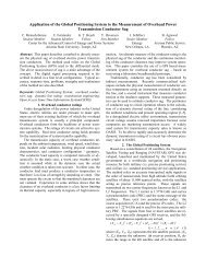
We proceed with the generalization for multiple-line outages
by next considering the case of the outages of the two
lines %l 1
and %l 2
.We simulate the impacts on , by introducing
ς % l
k
f l k
, taking explicitly into account the inter-
w ( l % 1
) and w ( l % 2
)
actions between these two transactions in specifying ∆ t( l % 1
)
and ∆ t( l % ) , as shown in Fig. 1. We set ∆ t( l % ) to satisfy
2
( ) ( ) ( ) ( )
w( % )
( ) ( %l
l ) 2
1 l%
2
1− ϕ % ∆ t %l
1
= f
l
% l .
(7)
1 1
Analogously, we select t( )
∆ l % 2
to satisfy
w( % )
( ) ( %l
l ) 1
2 l%
1
1− ϕ % ∆ t %l
2
= f
l
% l .
(8)
( ) ( ) ( ) ( )
2 2
We rewrite (7) and (8) using the relations in (3) and (4) as
⎡ ⎡ w %
( 1) w( 2 )
ϕ
l
l%
ϕ ⎤ ⎤ ⎡ t( 1 ) ⎤ % % ∆ %l ⎡ f %
⎢ ⎢ ⎤
l1 l1
⎥
l 1
I − ⎥ ⎢ ⎥
w( %
1) w( %
2 )
= ⎢
ϕ ϕ t ( 2 )
f
⎥ (9)
⎢ ⎢ l
l
⎥⎥
⎢∆
%l ⎥ ⎢ %l
⎣ 2
⎢ % ⎥⎦
.
⎣ ⎣ l
%
2 l 2 ⎦⎥⎦
⎣ ⎦
As long as the matrix in (9) is nonsingular, we determine
t ∆ t l % by solving the linear system.
∆ ( l % ) and ( )
1
2
Fig. 1. The impacts of the transactions w (% l ) and w (% )
1 l .
2
In the inductive process to generalize the result for the case
of multiple-line outages, we assume that the impacts of a set of
L % α −1 = l % 1, Ll , %
α−1
are simulated with
a−1 outaged lines ( ) { }
a−1 transactions whose amounts are specified by
⎡I − F
( 1) ( α −1 ⎣
∆ α − ) =
L % ⎤ t f
⎦
( α −1)
, (10)
where, ∆ t ( α −1 ) = ⎡∆ (% ) , K,
∆ ( l%
)
T
⎣ t l t ⎤
1
α−1
⎦ , f f , , f
( α 1 %
) ⎣
K
l %
1 lα−1
w( % l1) w( l%
α−1)
ϕ ⎤
% L
l
%
1 l1
⎥
M O M ⎡⎣
I − L%
⎤
α −1 ⎦
w( % l1) w( l%
α−1)
ϕ ⎥
% L
l
%
α−1 lα
−1
1
− =⎡ ⎤⎦
⎡ϕ
⎢
and F L % =
( α−1
) ⎢ ⎥ , with F nonsingular.
( )
⎢
⎣
ϕ
⎦
We now consider the additional line l% α∉L %
( α −1)
outage. The set
of outaged lines is L% ( ) = L% ( ) U{ l%
} . Reasoning along the
α α−1 α
lines used in the two-line outage analysis, ∆t ( α −1)
is given by
(
( )
) ( ) α
⎡
⎤
( ) ( ( ) ) ( ) α
⎣I − % l
l
F
α −1 ⎦ ∆ t α −1 = f
%
L %
α −1 . (11)
We capture the impacts of the outages of the L %( ) elements
on
t (% l 1 )
i
k
w( 1) w( 2)
f +∆ f % l
l
+∆f
%
l lk l
k k
i% j% i%
1
1 2
w( 1) w( 2
f +∆ f % l
l
+∆f
% )
% l1 l% %
1 l1
α −1
%l α
by using the analogue of (8) and determine t( α
)
( )
( ) ( L% )
( %
w %l
α −1 L
( α 1)
)
α
−
1−
ϕ
∆ t %l f
α = %l .
%l
α
α
( ) ( ) ( )
( )
( )
∆ % l from
T
(12)
The superscript L %
( )
denotes the network with the
α −1
j
k
t (% l 1 )
j%
2
t (% l 2 )
w( 1) w( 2
f +∆ f % l
l
+∆f
% )
% l 2 l% %
2 l 2
t (% l 2 )
elements of L %( ) outaged. We define
α −1
w( % l ) w( %
α
lα
)
b @ ⎡ϕ
,.., ϕ ⎤ ⎣ l% %
1 lα
−1
⎦
T
w
and
( l% 1) w( l%
⎡
1)
ϕ ,.., ϕ
α −
c @
⎤ and rewrite (11) and (12) as
% %
⎣ lα
lα
⎦
−1
w( %l α )
T
⎡⎣
I −F
L% ( )
⎤
1 ( 1)
( 1 ) ( f
α α ϕ
− ⎦
∆t − − b − + c ∆ t( α−1)
) = f
l% ( 1)
α l%
α −
α
(13)
w( %l α )
−1
( 1 −ϕ
) ∆t( % T
% lα
) −c ⎡ − ⎤
( )
( ( ) ( ))
1
1 t α f ,
α
⎣
I F %
α−
⎦
f α − + b ∆ l%
=
l
L
% lα
which may be simplified to
⎡ % b ⎤
( α −1)
⎡I −F % ⎤∆ t
( α ) ( α ) = f
⎣ L
⎦
( α )
, % @ F L
F ⎢
w( %
L α ) ⎥
( α )
T
l (14)
⎣
c ϕ %l α ⎦ .
So long as ⎡I −F L%
⎣
⎤
( α ) ⎦ is nonsingular, we use (14) to solve for
∆t and so simulate the impacts of the α line outages.
( α )
This development for specifying the appropriate values of
the transactions is used to provide the GLODF expression. For
any line k ∉ %
( L ( α)
)
l L ( ) , we define ξ %
, whose elements are the
α
GLODFs with the lines in L %
( ) outaged, with the interactions
α
between the outaged lines fully considered. The change in the
real power flow of line l is
k
( f l )
l k
T
( )
∆ @ ⎡ξ
⎤
⎣ ⎦ f
k
( L% ( α ) ) L%
( α )
lk
l ∉ L % (15)
( α )
, k ( α )
However, the combined impacts on line l of the a
k
transactions with the ∆t ( α ) specified by (14) is
( L% ( α ) ) w( l% 1 ) w( l%
α )
( ∆ f ) = ⎡ϕ
, , ϕ ⎤ ∆
k ⎣
K
k k ⎦
t
l l l
( α )
. (16)
Therefore, for ⎡⎣
I −F L%
⎤
( α ) ⎦ nonsingular, we rewrite (16) as
( L%
( ) ) −1
α
w( 1 ) w( α )
( ∆ f ) = ⎡ϕ
l % l%
, , ϕ ⎤ ⎡I
− % ⎤
l k ( α )
k k ⎣ ⎦
f
( α
⎣
L
F L . (17)
l l ⎦
)
( L ( α)
)
It follows from (15) that is the solution of
ξ %
l k
F ( ) ( ) ( )
, (18)
T L% T
( α )
w l% 1
w l%
α
⎡⎣I
− L%
ξ = ⎡
( α )
⎤⎦ ϕ , , ϕ ⎤
l k ⎣ l L
k l k ⎦
and is defined whenever ⎡I −F L%
⎣
⎤
( α ) ⎦ is nonsingular. The case
for singular ⎡I −F L%
⎣
⎤
( α ) ⎦ indicates that the outage of the α
lines in L %
( ) separates the system into two or more islands.
α
The analysis of such cases is treated in [6]. In fact, a simple
case is the outage of a line whose PTDF equals one. In this
case, the outage of the line results in the creation of two
separate subsystems. When the outaged line whose PTDF is
unity happens to be a radial tie, the outage results in the
isolation of the radial node.
The relation (18) provides an analytic, closed-form
expression for the GLODFs. Since the GLODF is expressed in
terms of the pre-outage network parameters, we avoid the need
to evaluate the post-outage network parameters. A key
advantage in the deployment of GLODFs is the ability to
evaluate the post-outage flows on specific lines of interest
without the need to determine the post-outage network states.
The proposed LODF extension permits the GLODF evaluation
through a computationally efficient procedure which involves
the solution of a system of linear equations whose dimension is
T

3
is the number of line outages.
IV. SUMMARY
The prominent role of cascading outages in recent blackouts
has created a critical need in security applications for the rapid
assessment of multiple-line outage impacts. We developed a
closed-form analytic expression for GLODFs under multiple-line
outages without the reevaluation of post-outage network
system parameters. This general expression allows the
computationally efficient evaluation of GLODFs for security
application purposes. A very useful application of GLODFs is
in the detection of island formation and the identification of
causal factors under multiple-line outages [6].
REFERENCES
[1] A. Wood and B. Wollenberg, Power Generation Operation and
Control, 2nd edition, New York: John Wiley & Sons, p.422, 1996.
[2] R. Baldick, “Variation of distribution factors with loading,” IEEE
Trans. on Power Syst., vol. 18, pp. 1316–1323, Nov. 2003.
[3] F.D. Galiana, “Bound estimates of the severity of line outages,”
IEEE Trans. on Power Apparatus and Systems, vol. PAS-103, pp.
2612–2624, Feb. 1984.
[4] M. Liu and G. Gross, “Effectiveness of the distribution factor
approximations used in congestion modeling”, In Proceedings of the
14th Power Systems Computation Conference, Seville, 24-28 June,
2002.
[5] M. Liu and G. Gross, “Role of distribution factors in congestion
revenue rights applications,” IEEE Trans. on Power Syst., vol. 19,
pp. 802-810, May 2004.
[6] T. Guler and G. Gross, “Detection of island formation and
identification of causal factors under multiple line outages,” to be
published in IEEE Trans. on Power Syst.