Induction Motor Load Dynamics: Impact on Voltage Recovery ...

4
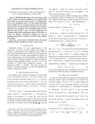
load data. The model supports two mechanical loading
modes: (a) Torque equilibrium (steady state), and (b) Constant
Slip.
~
I dk
BUS k
r 1 jx 1
r 2 jx 2
r 2
( 1- s n )
En
~
jx m
Fig. 4. <strong>Induction</strong> motor equivalent circuit.
1
r 1 + jx 1
1
jx m
1
r 2 + jx 2
= g 1 +jb 1
= jb m
= g 2
+jb 2
Circuit analysis of the induction motor equivalent circuit
yields the equations:
~
~ ~
I
dk
( g1
jb1
)( Vk
En
)
~ ~ sn
~ ~
(4)
0 jbm
En
En
( g1
jb1
)( Vk
En
)
r jx s
2
2
n
An additional equation links the electrical state variables to
the mechanical torque produced by the motor. This equation
is derived by equating the mechanical power (torque times
mechanical frequency) to the power consumed by the variable
resistor in the equivalent circuit of Fig. 4.
T
1 s
2 n
em s
( 1 sn
) I r
(5)
2 2
sn
or
~
0 T
(6)
2
En
snr2
r2
jx2sn
where
S
n
: induction motor slip,
T : mechanical torque produced by motor,
em
: synchronous mechanical speed.
s
em
s
Two compact models are defined from the above equations:
(a) Constant Slip Model (Linear):
~
~
~
I
dk
( g1
jb1
) Vk
( g1
jb1
) En
~
0 (
g jb ) V ( g jb jb
1
1
k
1
1
m
sn
~
) En
r jx s
In the constant slip mode the motor operates at constant speed.
The value of the slip is known from the operating speed and
therefore the model is linear. The terminal voltage V ~ and the
k
internal rotor voltage E ~ are the states of the model. Note that
n
the equations are given in compact complex form. In real
2
2
n
s n
(7)
form, separating real and imaginary parts yields a system of
four linear equations. The state vector is defined as
T
x V
kr
Vki
Eni
Enr
, where the subscripts r and
i denote real and imaginary parts respectively.
(b) Torque Equilibrium Model (Nonlinear):
~
~ ~
I
dk
( g1 jb1
)( Vk
En
)
~ ~ sn
~ ~
0 jbmEn
En
( g1
jb1
)( Vk
En
) (8)
r2
jx2sn
~ 2
En
0 snr2
Tems
r jx s
2
2
n
In the torque equilibrium model the slip is not constant and
thus it becomes part of the state vector. Note that this model is
nonlinear and not quadratic since the second and third
equations contain high order expressions of state variables. In
order to quadratize the model equations, we introduce three
additional state variables, namely Y ~ n
, W ~ ,
n
U
n
defined as
follows:
~ 1
Yn
(9)
r2
jx2sn
~ ~ ~
Wn
YnEn
(10)
~ ~ *
U W W
(11)
n
n
n
The state vector in this mode is defined as:
T ~ ~
~ ~
x V E s jU Y W .
k
n
n
n
n
The quadratic model equations are:
~
~
~
I
dk
( g1
jb1
) Vk
( g1
jb1
) En
~
~ ~
0 (
g1
jb1
) Vk
( g1
j(
b1
bm
)) En
Wnsn
0 Tem s
U
nsnr2
(12)
~ ~ *
0 WnWn
U
n
~ ~
0 r2Y
n
jx2snYn
1
~ ~ ~
0 W Y
E
n
n
n
The first equation gives the stator current of the motor; the
second equation comes from the equivalent circuit analysis;
the third equation specifies the torque produced by the motor.
The last three equations introduce the new variables for the
quadratization. Note again that the state vector and the
equations are given in compact complex format. They are to
be expanded in real and imaginary parts to get the actual real
form of the model. Note also that the third and fourth
equations are real, and, therefore, the model has ten real
equations and states.
The described motor model, in both operating, modes, can
be immediately expressed in the generalized component form
of (1) and therefore incorporated in the SPQPF formulation.
The model equations are linear in the constant slip mode and
n