Induction Motor Load Dynamics: Impact on Voltage Recovery ...

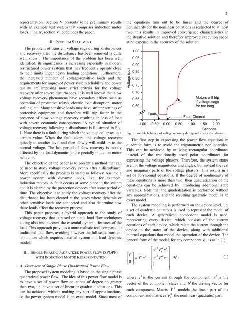
2
representation. Section V presents some preliminary results
with an example test system that comprises induction motor
loads. Finally, section VI concludes the paper.
II. PROBLEM STATEMENT
The problem of transient voltage sags during .disturbances
and recovery after the disturbance has been removed is quite
well known. The importance of the problem has been well
identified; its significance is increasing especially in modern
restructured power systems that may frequently operate close
to their limits under heavy loading conditions. Furthermore,
the increased number of voltage-sensitive loads and the
requirements for improved power system reliability and power
quality are imposing more strict criteria for the voltage
recovery after severe disturbances. It is well known that slow
voltage recovery phenomena have secondary effects such as
operation of protective relays, electric load disruption, motor
stalling, etc. Many sensitive loads may have stricter settings of
protective equipment and therefore will trip faster in the
presence of slow voltage recovery resulting in loss of load
with severe economic consequences. A typical situation of
voltage recovery following a disturbance is illustrated in Fig.
1. Note there is a fault during which the voltage collapses to a
certain value. When the fault clears, the voltage recovers
quickly to another level and then slowly will build up to the
normal voltage. The last period of slow recovery is mostly
affected by the load dynamics and especially induction motor
behavior.
The objective of the paper is to present a method that can
be used to study voltage recovery events after a disturbance.
More specifically the problem is stated as follows: Assume a
power system with dynamic loads, like, for example,
induction motors. A fault occurs at some place in the system
and it is cleared by the protection devices after some period of
time. The objective it to study the voltage recovery after the
disturbance has been cleared at the buses where dynamic or
other sensitive loads are connected and also determine how
these loads affect the recovery process.
This paper proposes a hybrid approach to the study of
voltage recovery that is based on static load flow techniques
taking also into account the essential dynamic features of the
load. This approach provides a more realistic tool compared to
traditional load flow, avoiding however the full scale transient
simulation which requires detailed system and load dynamic
models.
III. SINGLE-PHASE QUADRATIZED POWER FLOW (SPQPF)
WITH INDUCTION MOTOR REPRESENTATION
A. Overview of Single Phase Quadratized Power Flow
The proposed system modeling is based on the single phase
quadratized power flow. The idea of this power flow model is
to have a set of power flow equations of degree no greater
than two, i.e. have a set of linear or quadratic equations. This
can be achieved without making any sort of approximations,
so the power system model is an exact model. Since most of
the equations turn out to be linear and the degree of
nonlinearity for the nonlinear equations is restricted to at most
two, this results in improved convergence characteristics in
the iterative solution and therefore improved execution speed
at no expense in the accuracy of the solution.
Voltage (pu)
1.00
0.95
0.90
0.85
0.80
0.75
0.70
0.65
0.60
Fault
Fault Cleared
<strong>Motor</strong>s will trip
if voltage sags
for too long
-1.00 -0.50 0.00 0.50 1.00 1.50 2.00
Seconds
Fig. 1. Possible behavior of voltage recovery during and after a disturbance.
The first step in expressing the power flow equations in
quadratic form is to avoid the trigonometric nonlinearities.
This can be achieved by utilizing rectangular coordinates
instead of the traditionally used polar coordinates for
expressing the voltage phasors. Therefore, the system states
are not the voltage magnitudes and angles, but instead the real
and imaginary parts of the voltage phasors. This results in a
set of polynomial equations. If the degree of nonlinearity of
these equations is more than two, then quadratization of the
equations can be achieved by introducing additional state
variables. Note that the quadratization is performed without
any approximations, and the resulting quadratic model is an
exact model.
The system modeling is performed on the device level, i.e.
a set of quadratic equations is used to represent the model of
each device. A generalized component model is used,
representing every device, which consists of the current
equations of each device, which relate the current through the
device to the states of the device, along with additional
internal equations that model the operation of the device. The
general form of the model, for any component k , is as in (1)
k
i
Y
0
k
x
k
x
x
k T
k T
k k
F x
1
k k
F x b , (1)
2
k
i is the current through the component,
x k is the
where
vector of the component states and b k the driving vector for
each component. Matrix Y k models the linear part of the
component and matrices F the nonlinear (quadratic) part.
k
i