Visualization and Animation of Inverter-Driven Induction Motor ...

Proceedings of the 35th Hawaii International Conference on System Sciences - 2002
Visualization and Animation of Inverter-Driven Induction Motor
Operation
A. P. Sakis Meliopoulos, W. Gao
Electrical and Computer Engineering
Georgia Institute of Technology
Atlanta, Georgia 30332
Sakis.Meliopoulos@ece.gatech.edu
Abstract: This paper discusses a new model of an inverterdriven
induction motor that enables direct animation and
visualization of the inverter and motor operation. The models
of the inverter and induction motor are physically based
model in actual quantities. As such they enable direct
animation and visualization of the operation of the inverterdriven
induction motor. The paper discusses the models and
the animation and visualization approach. Specifically, the
animation and visualization screens are discussed in terms of
the displayed information. The implementation is in Open GL
that permits rendering as well as rotation, panning, and
zooming in real time. The paper presentation is by means of a
live presentation of the animation and visualization models.
Introduction
Inverter-driven induction motors have many advantages: (a)
use of rugged and inexpensive induction motors without the
disadvantage of high starting currents, and (b) speed control
over a wide range, and (c) economic operation in applications
of variable speed. Intensive research activities focus on
improvements of inverter-driven induction motors. This
research can be facilitated with high fidelity models of these
systems and animation and visualization methods. This paper
presents such an approach.
The paper first presents the computational engine, the model
of the inverter-driven induction motor and the approach
towards the animation and visualization. Specific examples
are provided.
The Virtual Power System Concept
Recent advances in software engineering have made it
possible to develop dynamic system simulators that operate in
a multitasking environment. The addition of graphical user
interface tools and hardware-accelerated graphics make the
final product an indispensable tool to the understanding of the
operation of the system. Many products have been developed
along these lines for power system engineering. Most of these
are focused on simulating the system under sinusoidal steady
state operation. Projecting the capabilities of the new
technologies, claims of replacing physical laboratories with a
virtual environment have surfaced. A virtual laboratory
should have the following features:
George J. Cokkinides
Electrical and Computer Engineering
University of South Carolina
Columbia, SC 29208
1. Continuous simulation of the system under study.
2. Ability to modify the system under study during the
simulation, and immediately observe the effects of
the changes.
3. Provide advanced output data visualization options
such as animated 2-D or 3-D displays that illustrate
the operation of any device in the system under
study.
The above properties are fundamental for a virtual
environment. The first property guarantees the uninterrupted
operation of the system under study in the same way as in a
physical laboratory: once a system has been assembled, it will
continue to operate. The second property guarantees the
ability to connect and disconnect devices into the system
without interrupting the simulation of the system. This
property duplicates the capability of physical laboratories
where one can connect a component to the physical system
and observe the reaction immediately. For example
connecting a motor to the power supply and observing the
startup transients, etc. The third property duplicates the
ability to observe the simulated system operation, in a similar
way as in a physical laboratory.
In principle, the minimal requirements of a virtual
environment can be achieved with present software and
hardware technology. However, this task is nontrivial. For
example, simulation methods that will accurately capture the
system response under all possible conditions require wide
band models for all power system components. This fact
becomes apparent if one considers specific examples such as
a power transformer. Nevertheless the technology exists to
achieve all three requirements of a virtual environment. On
the other hand, once a virtual environment has been
developed, it can be of greater educational value than a
physical laboratory. For example, in a physical laboratory we
are limited as to what we can directly observe. Consider an
electric motor. In a physical laboratory we can observe the
motor speed, measure the torque etc., but we cannot observe
the inner workings of the motor, magnetic field distribution
and interaction, small rotor oscillations, etc. A virtual
laboratory can provide this information using appropriate
visualization techniques. In a physical laboratory, most fast
transients will be missed because of limitations in human
observability speed. A virtual laboratory can provide this
capability. For, example, the operation of the system can be
1
0-7695-1435-9/02 $17.00 (c) 2002 IEEE 1

GUI
ACF
Proceedings of the 35th Hawaii International Conference on System Sciences - 2002
slowed down or paused and restarted to study a specific fast
transient condition.
In the past few years, we have undertaken an effort to explore
the development of a virtual simulation environment. The
central piece of this effort is a time domain simulator of
dynamical systems in a multitasking environment. In this
environment, visualization objects have access to the
instantaneous conditions of the components and the overall
system. Thus detailed 3-D “movies” of the instant-by-instant
operation of the component or the system can be generated.
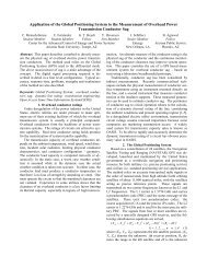
This paper presents the application of this technology to
inverter-driven induction motors.
The paper provides a brief overview of the new tool, the
mathematical formulation of the simulator and the data flow
between the time domain simulator and the visualization
objects. The paper focuses on the inverter-driven induction
motor. It presents the modeling of this system and the
approach towards the animation and visualization of this
system.
Description of the Virtual Power System
Environment
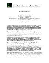
The internal structure of the Virtual Power System
environment is illustrated in Figure 1. This architecture was
developed with consideration on the minimal representation
of system components and the requirements of a virtual
environment. In the background is the network solver that is
a time domain simulation program. The network solver is
based on the representation of each system component with
its algebraic companion form (ACF) [1]. The ACF is
developed from the integro-differential equations of a
component by numerical integration. The ACFs of all
components in a system are related via the connectivity
constraints. Application of the connectivity constraints yields
a quadratic network equation that is solved at the network
solver.
Composite Model Object
The network solver is continuously executed providing the
simultaneous solution of the entire system and determines the
state of each component of the system. This information is
passed back to the individual devices for animation and
visualization of a specific component or groups of
components. The Virtual Test Bed has been developed in a
multitasking environment, thus allowing parameter changes
and immediate system response observations.
Any power system component can be modeled in such a way
that it can be interfaced with the Virtual Power System.
Appendix A describes the procedure for an induction
machine. The point is made that the model development of
the induction machine is physically based, i.e. the stator as
well as the rotor are explicitly represented in their own
variables, in other words no convenient transformations are
used. This is important for animation and visualization since
the actual physical quantities can be displayed. In the case of
the induction motor, one can observe the frequency of the
rotor currents and how it changes as the induction machine
accelerates or decelerates. The inverter model is also
similarly modeled.
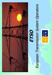
Example System
This example illustrates the dynamics associated with an
inverter-driven induction motor. The overall system is
illustrated in Figure 2. It consists of a source, a transmission
line, a transformer, a rectifier, an inverter and an induction
machine and the mechanical load of the induction motor.
G
A
A
A
BUS10 BUS20 BUS480
DCBUS
MOTOR
V
V
A
A
V
V
V
1 2
V
V
V
IM
SHAFT
Initialization
Re-Initialization
Time-Step
SVD/Numerical Stability
Network
Solver
TransMatrix/SSS
Analysis
Phasor/QSS
Analysis
Figure 2. Example System of Inverter-Driven Induction
Motor and Mechanical Load
V
Schematic Icon
Visualization Module
Schematic
Editor
Visualization
Engine
Figure 1. The Virtual Test Bed Architecture
The figure illustrates a number of meters that monitor various
physical quantities of the system, i.e. speed, torque and
voltage versus time plots. In addition to these graphs, two
animation objects are included which show the operation of
the inverter and the operation of the induction motor in an
animated way. A snapshot of the animation is shown in
Figures 3 and 4.
2
0-7695-1435-9/02 $17.00 (c) 2002 IEEE 2

Proceedings of the 35th Hawaii International Conference on System Sciences - 2002
simulation progresses so as to provide the animation. The
entire display can be rotated, panned and zoomed as the
simulation progresses to view the evolution of the state of the
induction motor from all possible angles. Similar animations
can be provided for other physical quantities of the motor.
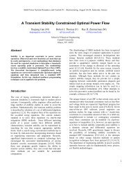
Figure 3. A Snapshot of the Animation of the Inverter
Showing the Voltage Distribution Along the Circuits of
the Inverter.
It is important to note that the system is multitasking allowing
multiple animations of the same system. For example one can
create an animation of the inverter showing the inverter
voltages, another animation of the inverter currents and
another animation of the motor position, torque and magnetic
fluxes. All these animations can be simultaneously viewed on
three different windows.
Conclusions
The technology for the development of virtual power system
laboratories was demonstrated. However, much more work
remains to develop a comprehensive library of visualization
modules for the plethora of existing power system elements.
We have discussed our recent work towards the development
of a virtual simulation environment and presented a specific
application example of an inverter-driven induction motor. It
is clear that virtual laboratories can be quite beneficial from
the educational point of view as they can provide insight of
the system under study that are impossible in a physical
laboratory. The presentation of the paper includes a live
demonstration of the inverter-driven induction motor
example.
Acknowledgments
The work reported in this paper has been partially supported
by the ONR Grant No. N00014-96-1-0926. This support is
gratefully acknowledged.
Figure 4. A Snapshot of the Animation of the Induction
Motor Operation Showing Torque, the Voltage
Distribution Along the Circuits of the Inverter
Figure 3 shows a screen snapshot in which the voltage
distribution along the circuits and components of the inverter
are displayed with a graph perpendicular to the plane of the
inverter. Note that the inverter is represented as a circuit in a
plane. The overall display can be rotated, panned and zoomed
as the simulation progresses to view the evolution of the
voltages from all possible angles. Similar animations can be
provided for the electric current
Figure 4 illustrates a snapshot of the induction motor
operation. Note that in this particular snapshot, the threedimensional
display of the induction motor is provided. The
rotor rotates as the simulation progresses. The torque, stator
magnetic flux, rotor magnetic flux and air gap magnetic flux
are illustrated on planes perpendicular to the motor axis. The
displays of these quantities are continuously updated as the
References
1. A. P. Sakis Meliopoulos and G. J. Cokkinides, ‘’A Time
Domain Model for Flicker Analysis’, Proceedings of the
IPST ’97, pp. 365-368, Seattle, WA, June 1997.
2. Eugene V. Solodovnik, George J. Cokkinides and A. P.
Sakis Meliopoulos, “Comparison of Implicit and Explicit
Integration Techniques on the Non-Ideal Transformer
Example”, Proceedings of the Thirtieth Southeastern
Symposium on System Theory, pp. 32-37, West Virginia,
March 1998
3. Eugene V. Solodovnik, George J. Cokkinides and A. P.
Sakis Meliopoulos, “On Stability of Implicit Numerical
Methods in Nonlinear Dynamical Systems Simulation”,
Proceedings of the Thirtieth Southeastern Symposium on
System Theory, pp. 27-31, West Virginia, March 1998.
4. Beides, H., Meliopoulos, A. P. and Zhang, F. "Modeling
and Analysis of Power System Under Periodic Steady
State Controls", IEEE 35th Midwest Symposium on
Circuit and Systems
3
0-7695-1435-9/02 $17.00 (c) 2002 IEEE 3

Proceedings of the 35th Hawaii International Conference on System Sciences - 2002
5. A. P. Sakis Meliopoulos, Power System Grounding and
Transients, Marcel Dekker, Inc., 1988.
6. A. P. Sakis Meliopoulos, G. J. Cokkinides and A. G.
Bakirtzis, “Load-Frequency Control Service in a
Deregulated Environment”, Decision Support Systems,
Vol. 24, No. 3-4, pp. 243-250, January 1999.
7. A. P. Sakis Meliopoulos, Murad Asad and George J.
Cokkinides, ‘Issues of Reactive Power and Voltage
Control Pricing in a Deregulated Environment’,
Proceedings of the 32 st Annual Hawaii International
Conference on System Sciences, p. 113 (pp. 1-7), Wailea,
Maui, Hawaii, January 5-8, 1999.
8. Ben Beker, George J. Cokkinides, Roger Dugal and A. P.
Sakis Meliopoulos, ‘The Virtual Test Bed for PEBB
Based Systems’, Proceedings of the 3rd International
Conference on Digital Power System Simulators,
Vasteras, Sweden, May 25-28, 1999.
9. A. P. Sakis Meliopoulos, David Taylor, George J.
Cokkinides and Ben Beker ‘Small Signal Stability
Analysis in PEBB Based Systems’, Proceedings of the
3rd International Conference on Digital Power System
Simulators, Vasteras, Sweden, May 25-28, 1999.
10. A. P. Meliopoulos and George J. Cokkinides ‘Small
Signal Stability Analysis in PEBB Driven Motion
Systems’, Proceedings of the ELECTROMOTION ’99
Symposium, pp. 273-278, Patras, Greece, July 8-9, 1999.
Biographies
A. P. Sakis Meliopoulos (M '76, SM '83, F '93) was born in
Katerini, Greece, in 1949. He received the M.E. and E.E.
diploma from the National Technical University of Athens,
Greece, in 1972; the M.S.E.E. and Ph.D. degrees from the
Georgia Institute of Technology in 1974 and 1976,
respectively. In 1971, he worked for Western Electric in
Atlanta, Georgia. In 1976, he joined the Faculty of Electrical
Engineering, Georgia Institute of Technology, where he is
presently a professor. He is active in teaching and research in
the general areas of modeling, analysis, and control of power
systems. He has made significant contributions to power
system grounding, harmonics, and reliability assessment of
power systems. He is the author of the books, Power Systems
Grounding and Transients, Marcel Dekker, June 1988,
Lightning and Overvoltage Protection, Section 27, Standard
Handbook for Electrical Engineers, McGraw Hill, 1993, and
the monograph, Numerical Solution Methods of Algebraic
Equations, EPRI monograph series. Dr. Meliopoulos is a
member of the Hellenic Society of Professional Engineering
and the Sigma Xi.
George Cokkinides (M '85) was born in Athens, Greece, in
1955. He obtained the B.S., M.S., and Ph.D. degrees at the
Georgia Institute of Technology in 1978, 1980, and 1985,
respectively. From 1983 to 1985, he was a research engineer
at the Georgia Tech Research Institute. Since 1985, he has
been with the University of South Carolina where he is
presently an Associate Professor of Electrical Engineering.
His research interests include power system modeling and
simulation, power electronics applications, power system
harmonics, and measurement instrumentation. Dr. Cokkinides
is a member of the IEEE/PES.
W. Gao was born in Jiangxi, China in 1968. He received the
Bachelor degree in Engineering from Northwestern
Polytechnic University, Xi’an, China, in 1988; the Master
degree in industrial automation from Northeastern University,
Shenyang, China, in 1991. He is currently working for his
Ph.D. degree in the School of Electrical and Computer
Engineering in Georgia Institute of Technology.
Appendix A: Induction Motor Model
The dynamic equations of the electrical system of an induction
machine are derived in this section. The induction machine can
be viewed as a set of mutually coupled inductors, which
interact among themselves to generate the electromagnetic
torque. Straightforward circuit analysis leads to the derivation
of an appropriate mathematical model.
ω m
θ r
(t)
phase a
magnetic axis
reference
i as
(t) v as
(t)
r i
as
s
(t)
v a′ s
(t)
i ar
(t)
v ar
(t)
i a′ r
(t) v a′ r
(t)
r v cr
(t)
ar
i cr
(t)
i v c′ r
(t)
c′ r
(t)
i br
(t)
v br
(t)
v
i r
(t)
b′ r
(t)
b′
i cs
(t) v cs
(t
i c′ s
(t) v c′ s )
i bs
(t)
v bs
)(t )
a′
b′
)
)
i s
(t
v s
(t b′
Figure 1. A general induction machine as a set of
mutually coupled windings
In the process of derivation, the following assumptions are
made: (1) the machine is cylindrical; (2) space mmf and flux
waves are sinusoidally distributed (neglecting the teeth and
slots effects); (3) the saturation, hysteresis, and eddy currents
are neglected. Figure 1 illustrates the stator and rotor
windings of an induction machine: three phase stator
windings, and three phase rotor windings. The rotor may be
4
0-7695-1435-9/02 $17.00 (c) 2002 IEEE 4

Proceedings of the 35th Hawaii International Conference on System Sciences - 2002
wound rotor or squirrel cage rotor. In either case, the rotor
windings can be idealized in the same way as the stator
windings. In fact, there is a procedure for representing the
squirrel cage by an equivalent set of sinusoidally distributed
windings. Note that all inductors are mounted on the same
magnetic circuit and thus they are all magnetically coupled.
The position of the rotating rotor is denoted with the
electrical angle between the stator phase as magnetic axis (a
stationary reference) and the rotor phase ar magnetic axis,
θ
r
(t) . The mechanical rotor position angle is:
2
θ
m( t)
= θr
( t)
(A.1)
p
where p is the number of poles of the rotating magnetic field
in the air gap.
Application of Kirchhoff's voltage law to the circuit of Figure
1 yields:
d
vabcs( t)
− va'
b'
c'
s(
t)
= Rsiabcs
( t)
+ λabcs
( t)
(A.2)
dt
d
vabcr
( t)
− va'
b'
c'
r
( t)
= Rriabcr
( t)
+ λabcr
( t)
(A.3)
dt
i
a'
b'
c'
s
i
a'
b'
c'
r
( t)
= −i
( t)
(A.4a)
abcs
( t)
= −i
( t)
(A.4b)
abcr
where
v ( t)
= v ( t)
v ( t)
v ( t)
[ ] T
abcs
as bs cs
[ ] T
abcr
( t)
= var(
t)
vbr
( t)
vcr
( t
[ ] T
abcs
( t)
= ias
( t)
ibs
( t)
ics
( t
[ ] T
abcr
( t)
= iar
( t)
ibr
( t)
icr
( t
[ ] T
a' b'
c'
s
( t)
= va'
s
( t)
vb
' s(
t)
vc'
s
( t
[ ] T
a' b'
c'
r
( t)
= va
' r
( t)
vb
' r
( t)
vc
' r
( t
[ ] T
a' b'
c'
s( t)
= ia'
s
( t)
ib'
s(
t)
ic
' s(
t
[ ] T
a' b'
c'
r
( t)
= ia'
r
( t)
ib
' r
( t)
ic
' r
( t
[ ] T
abcs
( t ) = λ
as
( t)
λbs
( t)
λ
cs
( t)
[ ] T
abcr
( t ) = λ
ar
( t)
λbr
( t)
λ
cr
( t)
s
diag( ras
rbs
rcs
)
r
diag( rar
rbr
rcr
)
= [ 1 1 1] T
v )
i )
i )
v )
v )
i )
i )
λ
λ
R =
R =
Γ
λ
abcs
(t) is the vector consisting of the magnetic flux
linkages of stator phase as, bs, and cs, respectively. λ
abcr
(t)
is the vector consisting of the magnetic flux linkages of rotor
phase ar, br, and cr, respectively. Note that if
R = diag
s
R = diag
r
( r r r )
s
s
( r r r )
r
r
s
r
then, we have balanced rotor windings and stator windings.
In Equations (A.2) and (A.3), the magnetic flux linkages are
complex functions of the rotor position and the electric
currents flowing in the various windings of the machine. The
magnetic flux linkages of the phase a, b, and c are:
⎡λ
⎢
⎣λ
( t)
⎤ ⎡ Lss
⎥ =
( t)
⎢
⎦ ⎣Lrs
( t)
(2.5)
abcs
abcr
where
⎡Lls
+ L
⎢ 1
L
ss
=
⎢
−
2
L
⎢
1
⎣ −
2
L
L
rr
L ( t)
= L
sr
ms
ms
⎡Llr
+ L
⎢ 1
=
⎢
−
2
L
⎢
1
⎣ −
2
L
sr
mr
mr
ms
mr
L
−
ls
−
L
⎡ cos( θr
( t))
⎢
⎢
cos( θ ( t)
−
2
r
⎢⎣
cos( θ ( t)
+
2
r
L
−
lr
−
π
3
π
3
)
)
Lsr
( t)
⎤⎡i
L
⎥⎢
rr ⎦⎣i
1
2
+ L
1
2
1
2
L
L
ms
ms
+ L
1
2
L
L
ms
mr
mr
mr
T
( t)
L ( t)
rs
=
cos( θ
abcs
abcr
( t)
⎤
( t)
⎥
⎦
1
−
2
Lms
1
−
2
Lms
L + L
ls
ms
1
−
2
Lmr
1
−
2
Lmr
L + L
lr
cos( θ ( t)
+
r
cos( θ ( t)
−
sr
r
r
2π
3
( t))
2π
3
)
)
mr
⎤
⎥
⎥
⎥⎦
⎤
⎥
⎥
⎥⎦
cos( θ ( t)
−
2
r
cos( θ ( t)
+
2
r
cos( θ ( t))
The notation in above equations is obvious. ( L
ls
+ L ms
) is
the self-inductance for each of stator windings, and
the stator magnetizing inductance. ( )
lr
L mr
r
L is
L + is the selfinductance
for each of rotor windings, and L
mr
is the rotor
magnetizing inductance. L
sr
is the maximum mutual
inductance between a stator phase winding and a rotor phase
winding. Notice that the mutual inductances in matrix
ms
π
3
π
3
) ⎤
)
⎥
⎥
⎥⎦
5
0-7695-1435-9/02 $17.00 (c) 2002 IEEE 5

Proceedings of the 35th Hawaii International Conference on System Sciences - 2002
L sr
(t) are dependent on the position of the rotor, which is
time varying. This makes the overall system highly nonlinear
and time varying.
The electromagnetic torque is given by the equation:
Pem
( t)
dw
fld
( t)
Tem
( t)
= = . It determines the amount of
ωm
( t)
dθm
power converted from electrical power into mechanical
power and can be computed by differentiating the field
energy function w fld
(t)
with respect to the rotor mechanical
position θ
m
. In particular, we have:
T
em
⎛ ∂L
( t)
( t)
abcs
⎟ ⎞
=
⎜
abcr
t
⎝ ∂θ
m ⎠
T sr
( i ( t)
) ⎜ i ( )
Upon substitution and some manipulations, the rotor
equations are expressed in the form:
dω
( t)
T ⎛
m
∂L
( t)
⎞
sr
J = ( iabcs
( t)
) iabcr
( t)
− Tm
( t)
dt
⎜
⎟
⎝ ∂θm
⎠
(A.6)
dθ m
( t)
= ω
m
( t)
dt
(A.7)
6
0-7695-1435-9/02 $17.00 (c) 2002 IEEE 6