Simple analytical models of glacier-climate interactions - by Prof. J ...

h(x) =
2 τ 0
ρ g x for 0 ≤ x ≤ L 2 , (2.4)
h(x) =
2 τ 0
ρ g (L-x) for L 2 ≤ x ≤ L .
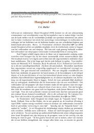
The profile is shown in Fig. 2.1 (in the example shown L = 200 km and
2 τ 0 / ρ g = 10 m). Although it provides a reasonable first approximation to the shape of
an ice cap, there are some deficiencies. First of all the solution is not valid close to the ice
divide, where the surface slope is very small and longitudinal stresses dominate;
therefore, here the ice flow cannot be approximated by plane shear. Secondly, a property
of the perfectly plastic ice cap is that, given the size, its thickness does not depend on the
mass balance. Although we will see later that this dependence is generally weak, in some
applications it is of importance. The ice velocity or mass flux is not directly related to the
profile, but can only be obtained from the conservation of mass. For instance, for one
half of the ice sheet:
H u =
L
L/2
b n dx
. (2.5)
In this equation u is the vertically averaged horizontal ice velocity and b is the specific
balance rate.
Next we consider the isostatic depression of the bed. A balance is present only when the
following condition is met (ρ i and ρ m are the ice and mantle density, respectively):
ρ i H + ρ m b = ρ i (h-b) + ρ m b = 0 . (2.6)
The height of the bed b then is (b < 0):
Fig. 2.1
1000
h (m)
750
500
250
0
0 50 100 150 200
x (km)
8