Simple analytical models of glacier-climate interactions - by Prof. J ...
Simple analytical models of glacier-climate interactions - by Prof. J ...
Simple analytical models of glacier-climate interactions - by Prof. J ...

Create successful ePaper yourself
Turn your PDF publications into a flip-book with our unique Google optimized e-Paper software.
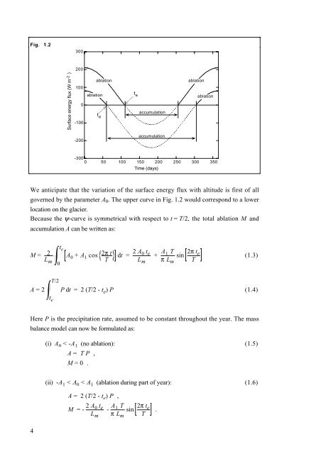
Fig. 1.2<br />
300<br />
200<br />
Surface energy flux (W m -2 )<br />
100<br />
0<br />
-100<br />
ablation<br />
ablation<br />
t e<br />
t e<br />
accumulation<br />
ablation<br />
ablation<br />
-200<br />
accumulation<br />
-300<br />
0 50 100 150 200 250 300 350<br />
Time (days)<br />
We anticipate that the variation <strong>of</strong> the surface energy flux with altitude is first <strong>of</strong> all<br />
governed <strong>by</strong> the parameter A 0 . The upper curve in Fig. 1.2 would correspond to a lower<br />
location on the <strong>glacier</strong>.<br />
Because the ψ-curve is symmetrical with respect to t = T/2, the total ablation M and<br />
accumulation A can be written as:<br />
M = 2<br />
Lm<br />
0<br />
t e<br />
A 0 + A 1 cos 2π t<br />
T<br />
dt<br />
= 2 A 0 t e<br />
L m<br />
+ A 1 T sin 2π t e<br />
π L m T<br />
(1.3)<br />
A = 2<br />
T/2<br />
P dt<br />
t e<br />
= 2 (T/2 - t e ) P (1.4)<br />
Here P is the precipitation rate, assumed to be constant throughout the year. The mass<br />
balance model can now be formulated as:<br />
(i) A 0 < -A 1 (no ablation): (1.5)<br />
A = T P ,<br />
M = 0 .<br />
(ii) -A 1 < A 0 < A 1 (ablation during part <strong>of</strong> year): (1.6)<br />
A = 2 (T/2 - t e ) P ,<br />
M = - 2 A 0 t e<br />
L m<br />
- A 1 T sin 2π t e<br />
π L m T<br />
.<br />
4