Simple analytical models of glacier-climate interactions - by Prof. J ...
Simple analytical models of glacier-climate interactions - by Prof. J ...
Simple analytical models of glacier-climate interactions - by Prof. J ...

You also want an ePaper? Increase the reach of your titles
YUMPU automatically turns print PDFs into web optimized ePapers that Google loves.
Note that values <strong>of</strong> L for which N < 0 are spurious and should not be considered.<br />
An example is shown in Fig. 6.1. Parameter values are: µ = 9 m, ν = 20, s = 0.06 .<br />
Because L = 0 is a stable solution for E ' > 0 (equilibrium line above the bed<br />
everywhere), there are two stable branches and one unstable branch (dotted). In terms <strong>of</strong><br />
catastrophe theory this model represents a fold, but because we add the condition that L<br />
should be positive it appears as a distorted cusp. The branching <strong>of</strong> the steady-state<br />
solutions that shows up here was in fact found numerically a long time ago (Oerlemans,<br />
1981). It should also be mentioned that the dynamics <strong>of</strong> the present <strong>glacier</strong> model are<br />
similar to those <strong>of</strong> a perfectly plastic ice sheet on a flat bed with a sloping equilibrium line<br />
Weertman (1961).<br />
The range <strong>of</strong> E '-values for which two stable solutions exist is<br />
0 ≤ E ' < E ' crit , (6.7)<br />
where the critical point E' crit is found <strong>by</strong> setting Det = 0:<br />
E ' crit =<br />
µ<br />
2 s (1 + ν s)<br />
. (6.8)<br />
Therefore, for increasing slope <strong>of</strong> the bed, the HMB-feedback becomes weaker and the<br />
critical point approaches the origin. The result for the linear <strong>analytical</strong> model is also<br />
shown. In this caseτ 0 /ρg was set to 9 m, because this is consistent with eq. (6.1) for<br />
s = 0. The squares in Fig. 6.1 shows the dependence <strong>of</strong> <strong>glacier</strong> length on E' as found <strong>by</strong><br />
a numerical plane-shear model for a <strong>glacier</strong> <strong>of</strong> constant width. Clearly, the nonlinear<br />
<strong>analytical</strong> model matches the numerical result very well.<br />
Fig. 6.1.<br />
14<br />
12<br />
10<br />
L (km)<br />
8<br />
6<br />
4<br />
linear model<br />
2<br />
0<br />
nonlinear model<br />
•<br />
•<br />
-200 -150 -100 -50 0 50<br />
E' (m)<br />
21