Diffusion frequency factors in some simple examples of transition ...

Proc. Nat. Acad. Sci. USA
Vol 73, No. 3, pp. 679-683, March 1976
Chemistry
Diffusion frequency factors in some simple examples of transitionstate
rate theory*
(Eyring rate theory/dynamics versus diffusion)
TERRELL L. HILL
Laboratory of Molecular Biology, National Institute of Arthritis, Metabolism, and Digestive Diseases, National Institutes of Health, Bethesda, Maryland 20014
Contributed by Terrell L. Hill, January 8, 1976
ABSTRACT In the Eyring rate theory, the rate constant
is expressed as a product of a frequency factor (kT/h) and a
quotient of partition functions. Continuing an earlier paper,
it is shown here by means of simple examples that the Eyring
formalism may be extended to include diffusion-controlled
processes if a new frequency factor, D/RA, is substituted for
kT/h, where D = diffusion coefficient, A = thermal de Broglie
wavelength, and R = a characteristic distance that depends
on the particular case. The Eyring formalism is also
applicable in hybrid cases, intermediate between diffusion
(D/RA) and dynamics (kT/h). Because these modified frequency
factors are not "universal" (as kT/h is), their main
use (other than conceptual) would appear to be in cases in
which one considers a simple model (with calculable frequency
factor) together with a related more complicated
model. In the latter case, as an approximation, one would
combine the "simple" frequency factor with the "complicated"
quotient of partition unctions in order to obtain the desired
rate constant. Examples are given.
In the Eyring rate theory, the rate constant is expressed as a
product of a frequency factor (f.f.) kT/h and a quotient of
partition functions (p.f.s), all relative to the same zero of energy
(1). It was shown in an earlier paper (2) that the Eyring
formalism can be extended to diffusion-controlled ligandmacromolecule
association in solution by substitution of a
new f.f., D/RA, in place of the usual dynamical factor
kT/h. The primary object in this paper is to supplement this
earlier discussion with additional elementary examples involving
diffusion. For completeness, we consider the corresponding
dynamical cases as well. Classical mechanics is
used throughout. The paper of Chandrasekar (3), following
Kramers (4), provides the necessary background and much
of the notation used.
ONE-DIMENSIONAL EXAMPLES
Diffusion Case. We consider the steady rate of transitions
in the direction A -- B for the case shown in Fig. 1 (3, 4),
where w = potential of mean force (1, 2). From the Smoluchowski
equation, Eq. 312 of ref. 3,
dc = j c-D -+ dw\
at ax' ax kT dx'
we obtain for the steady A -- B flux j (per unit area), as in
Eq. 472 of ref. 3,
= Dc 4e"- /IR [11
where
R fJ e-f(X/kTdX, [2]
Abbreviations: p.f., partition function; f.f., frequency factor.
*
This paper is dedicated to Henry Eyring as a personal "supplement"
to the recent volume [(1971) Advances in Chemical Physics,
eds. Prigogine, I. & Rice, S. (Wiley-Interscience, New York),
Vol. 211 published in his honor on the occasion of his seventieth
birthday.
D = diffusion coefficient, CA = local concentration at x =
XA, and f(X) - w w-w(X) in the neighborhood of x = xc.
The total number of particles (per unit area) in state A,
treated as at equilibrium, is nA = CAqAA, where qA = equilibrium
one-dimensional p.f. and A = h/(27rmkT)1/2 = thermal
deBroglie wavelength. This follows from the fact that
qAA is the so-called configuration integral (1) for state A.
For example (1, 3), qA = kT/hvA (classical harmonic oscillator).
The (first-order) rate constant for A A B is then (compare
Eq. 473 of ref. 3)
a = jI/nA = (DIRA)(e-w*1kT/qA) [3]
But since, for this simple model, q* = e-w*/kT in the Eyring
rate theory (1), we see again (2) that replacement of the f.f.
kT/h by a new factor D/RA produces the proper rate constant
in the diffusion case. Here, R is defined by Eq. 2. If we
expand f(X) about X = 0 and retain only the quadratic term
Wc2mX2/2, which defines wc, we find R = (2AkT/
If the barrier in w(X) has
Wc2m)1/2, or Wc2mR2/2 = 7rkT.
the hypothetical shape shown in the inset of Fig. 1, then R =
1. In either of these cases, for a wide barrier, i.e., R x, o we
have a D/RA - - 0.
As already pointed out (2), D/RA is not a "universal" f.f.
as kT/h is in the (generally somewhat approximate) Eyring
theory. Rather, D/RA depends on the special case. Despite
this, there are at least three advantages to rewriting diffusion
rate constants in the modified Eyring form, i.e., (DI
RA) X (p.f. quotient): (a) the considerable conceptual and
intuitive benefits deriving from the Eyring formalism are
thereby extended to a new class of rate processes; (b) it may
be possible to estimate R and hence to calculate the diffusion
rate constant (with the aid of the appropriate p.f.s) in some
cases in which the ab initio diffusion problem is too difficult
to solve; and (c) R may be found for a diffusion problem in
a relatively small number of coordinates (or the diffusion
problem might be simplified in some other way) and then
this R is retained, as an approximation, when more coordinates
are added to the model via the p.f.s.
An example of (c), above, has already been given (2):
translation A translation + rotation in the binding of spherical
ligands. Another example is in the paragraph following
Eq. 13 of ref. 2: R for the field-free binding case was retained,
as an approximation, for the case with an external
field (this approximation is not used below, in Eq. 24). As a
third example of (c), let us extend, formally, the one-dimensional
result in Eqs. 2 and 3 to three dimensions by allowing
yz-vibrational motion of the particle normal to the x-axis
(the "reaction coordinate"), both in the initial state and in
the transition state. Then
a= (DIRA)(q$ ,ze -u-*T/qAqA z)
[4]
where q*YZ and qAyz are the new vibrational p.f.s.
679

680 Chemistry: Hill
Proc. Nat. Acad. Sci. USA 73 (1976)
w
w=w* -f(X) s .w )) kT
w = 0 * - - - - -,
XA Xc XB
0 X = x -Xc
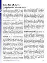
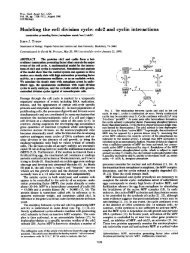
FIG. 1. Schematic. One-dimensional potential of mean force for study of transition A - B across barrier w* >> kT at xc. Inset shows
hypothetical barrier with flat top and steep edges.
General Relations. When (
=
kT/mD is not large compared
to 2wc, we need a solution of the (steady-state) Kramers
equation (Eq. 477, ref. 3)
wa + Kow =
OU aw + COW + qa0W
ax au auau
where W(X,u) = probability density in X and u (velocity), q
= kTf3/m, and K = -m-1dw/dX. We write
W(X,u) = CF(X,u)e-mu2/2kTee-w/kT [6]
where F 1 at equilibrium. Then (Eq. 485, ref. 3)
OF aF a2F aF
Ua + K a= - AlU u [7]
For the solution of Eq. 7 around the peak in w, the boundary
conditions are F = 1 for X - -c and F = 0 for X
+o. The required steady flux j across X = 0 (or, indeed,
across any other value of X) is
[5]
j= f W(X=o,u)udu. [8]
In the diffusion case 3>> 2wc and f = wc2mX2/2, we can
obtain j from§ Eqs. 6 through 8 (3), compare the result with
Eq. 1, and thus evaluate the normalization constant in W.
One finds C = cA(m/27rkT)'/2. Thus, the normalization is
such that, at equilibrium, fWdu = cAe-w/kT = local concentration.
Incidentally, in the diffusion case, one can show
from§ f Wdu at X = 0 (and verify from the Smoluchowski
equation approach) that the local concentration at the transition
state in steady flow is one-half the equilibrium value,
cAe/k
c -w*IkT
Dynamical Case. Here (3 = 0 and w = potential energy.
Only the left-hand sides of Eqs. 5 and 7 remain (Liouville's
equation). The solution, for our boundary conditions, is F =
1 or F = 0 with a step between these values along the curve
u = [2f(X)/m]'/2 in the X,u-plane. If f = WC2mX2/2, this
curve is the straight line u = wcX (Q = 0 in the notation of
ref. 3). On X = 0 (Eq. 8), where f = 0, F = 1 for u > 0 and
§ For this purpose, it is helpful to use (at X = 0) F(u) = ('k) + (Wc2/
27rfq)1/2u +.--.
F = 0 for u 0 and F = 0, u 1.5.
Thus, SYE and 5SD are merely two limiting forms of f.f.
(though no doubt the most important). Indeed, a further
generalization of considerable physical interest (which is
being investigated) follows on use of (3 = (3(X) in Eq. 7 instead
of (3 = constant. For example, ( is a step function: (3 =
(3- for X < 0 and (3 (3+ for X > 0 (see Discussion).
Of course a generalized 5' (i.e., one other than 9rE or 9'D)
can also be used in examples of type (c) above (see Eq. 29,
below).

0.8
0.6
0.4
0.2
X
Chemistry:
\1/2s
Hill
\ \
' \ ----
I-s ".
I...
0 1 2 3 4
s *l/2wc
-
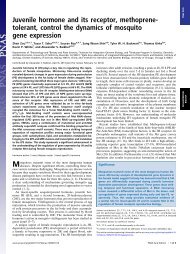
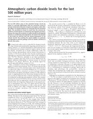
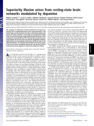
FIG. 2. Solid curve: /9E as a function of s = :X2wc (Eq. 12).
/E = 1 is the limiting value (O = kT/h) at s = 0; the initial slope
is -1. For large s, 9/E- 1/2s (i.e., 9 -. D = D/RA).
Finally, we note that, in the intermediate case, we also
have (M)cAe-w*/kT for the local concentration at X = 0,
since F(u) on X = 0 is equal to i plus an odd function of u.
THREE-DIMENSIONAL EXAMPLES (WITH
SPHERICAL SYMMETRY)
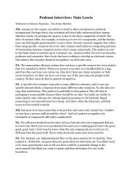
Bimolecular Association in Solution. We have already
considered (2) the case in which freely diffusing point (ligand)
particles may be bound at sites on relatively large adsorbent
molecules once a ligand molecule crosses a hemispherical
shell of radius rc (Fig. 3, dashed line) about any
site. It was found that, in the f.f. D/RA for this case, R = rc
(Eq. 9, ref. 2).
The above model can be modified easily to treat a bimolecular
reaction in which a molecule of species 1 (ml, Dl)
combines with another of species 2 (m2, D2) to form a bimolecular
complex whenever a mutual approach is made
within a critical distance rc. The second-order rate constant
a' for this process is found to be 47r(DI + D2)rc (Eq. 447,
ref. 3). The p.f.s involved are (ref. 1, p. 155)
q1 = V/A13, q2 = V/A23, q* = (V/A123)(27rkT/h2)4rrc2
[14]
where ml + M2 appears in A12 and 1A = Mlm2/(Ml + m2).
Proc. Nat. Acad. Sci. USA 73 (1976) 681
If, for this case, in view of the above paragraph, we write
the f.f. in the form (D1 + D2)/rcX, that is,
'= 47r(D, + D2)rc=
[(D1 + D2)/rcA](qt/V)/(q1/V)(q2/V) [15]
then we find, as one might expect, that X = h/(27rgukT)l/2.
If, say, species 2 is very large (M2 >> ml, D2

6.82 Chemistry: Hill
If w(r) has the simplified shape shown in inset (a) of Fig.
3, Eq. 18 gives R = rc, as found for the reverse processl (2).
If w(r) appears as in inset (b) of Fig. 3, we find R = rcl/(rc
+ 1).
A more realistic case: if w(r) = w* for r > rc (dashed line
in Fig. 3) and f = wC2mX2/2 for r < rc, then Eq. 18 gives R
rc + Ar, where Ar = (7rkT/2oc2m)'/2. The curvature
of f(r) for r < rc must be such that WCc2mrc2/2 = O(wt*) >>
kT. Therefore, rc >> Ar and R rc [i.e., essentially as in
the inset (a) case].
If, in Fig. 3, w* - WB >> kT and f = WC2mX2/2 on both
sides of r = rc (X = 0), then we get R n 2Ar, as already
found in the one-dimensional problem. Hence, the rate constant
for escape is much larger here than in the preceding
paragraph (R rc), the ratio being rc/2Ar.
-
Since we have now considered the diffusion-escape problem
in both one (Eq. 3) and three (Eq. 20) dimensions, we
can use the results to test, in a specific case, the approximation
suggested in Eq. 4. If we had started with Eq. 3 (for
present purposes, let us use RI to denote the R given by Eq.
2) and then introduced q yz = 27rrc2/A2 and qA- qAqAyz
into Eq. 4 in order to extend Eq. 3 to three dimensions, we
would have obtained Eq. 20 but with R1 in place of the correct
R3 (defined by Eq. 18). The approximation R1 - Rs is
satisfactory to the extent that one is justified in placing r-2
in Eq. 18 in front of the integral sign, as rc-2. Thus, the
sharper the peak in w(r), the better the approximation R1 _
R3. Indeed, we have already noted in the preceding paragraph
that, for the case f X2 (IXI > 0), R1 = 2Ar and R3
2Ar.
Finally, the concentration at r = rc (transition state) deserves
comment. If we take 1 = rA and 2 = rc in Eq. 16, we
find
= ce [1 - ( [22]
where the integrands are the same as in Eq. 18. Of course, if
there were equilibrium between the transition state and
state A, [ ] 1. In the "dashed line" case (Fig. 3) above, the
ratio f/f Ar/rc is small and [ ] 1. But in the next example
(f - X2 for Xi > 0), cc is one-half of the equilibrium
value cAe-w*/kT (as in the one-dimensional problem). For
insets (a) and (b) of Fig. 3, cc has the equilibrium value.
We turn now to the inverse (binding) process in the diffusion
case. Fig. 3 and Eq. 16 still apply except that now c
= 0 in state A and c = CB in state B (rB oo), If we choose
1 = rA and 2 = rB in Eq. 16, we obtain for the second-order
rate constant for binding ligand to macromolecule (2),
a' = -JICB = 2rDrc2e-(u- WB)/kT/R [23]
where R is again given by Eq. 18. The special cases of Fig. 3,
above, leading to various R values, apply here as well. For
example, for inset (a), a' = 27rDrc as in ref. 2, Eq. 8.
As already mentionedl, the f.f. D/RA in Eq. 20 must also
be involved here for the inverse process. But to verify this, a
little more care is required with the partition functions (because
the inverse process is bimolecular). Using qA and q2$
as defined above, we now write (2) p.f.A = qA3qV, p.f.$ =
q2tqV, qo = qV, and qB = (V/A3)e wB/kT, where qo is the
p.f. of a macromolecule with an empty binding site. Then
we find, as expected, that
a' = (D/RA)(p-f.*/V)/(q0/V)(qB/V) [24]
The f.f.s must necessarily be the same in the expressions for the
two inverse rate constants, in view of the p.f. ratios involved and
their relation to the equilibrium constant (1).
Proc. Nat. Acad. Sci. USA 73 (1976)
agrees with Eq. 23. The equilibrium constant for binding is
(compare Eq. 5, ref. 2)
K = a'/a = (pf-A/V)/(qO/V)(qB/V)
=
qA3A3ewRlkT. [25]
To find cc, we choose 1 = rA and 2 = rc in Eq. 16 with
the result
Cc = cBe-(u- WB)/kT (f/ ) [26]
In a certain sense, this is the inverse of Eq. 22. For insets (a)
and (b), Fig. 3, cc = 0. In the "dashed line" case, cc n
CBAr/rC, which is small. In the f X2 aIXI > 0) case, cc is
one-half of the equilibrium value.
_
In the conventional treatment of this binding problem,
using a differential equation in c, the boundary condition c
= 0 ("absorption") on the surface r = rc is used. The above
paragraph shows that this is usually safe (the cotrect condition
is CA = 0); however, in the f
- X2 case, c £ 0 is justified
only if w* - WB >> kT.
Dynamical Case. We consider the rate of escape, in Fig.
3, when 13 = 0. We are concerned with the three-dimensional
Liouville equation with potential energy w a function of r
only. But because of the condition rc >> Ar already mentioned
in relation to this figure, the spherical surface can be
treated as planar to a good approximation. Hence the discussion
of the one-dimensional dynamical case, above, applies
here with very little change. We obtain Eq. 9 for jr, as before,
for any shape f(r). The total flux across the surface r =
rc is J = 2lrrC2j,. The number of molecules in state A is nA
= cAqA3A3. Thus we are led to
a = J/nA = (kT/h)(q2t/qu), [27]
in agreement with Eyring's formulation (q2* is given by Eq.
21). If we use Eq. 19 for qA3,
a = VA(rc /rA)e [28]
Intermediate Case. For f = WC2mX2/2 and arbitrary f3/
2wc, again because of the condition rc >> Ar we have essentially
the one-dimensional differential equation, Eq. 5, to a
good approximation. The one-dimensional solution (3, 4)
can, therefore, be used but with J = 27rrC2j and nA =
cAqA3A3. Hence
al
[29]
= 3 (q2*/qA3)
where 5f is given by Eqs. 12 and 13. Note that this follows
from Eq. 11 simply by modifying the p.f. quotient. The
"exact" agreement in f.f. in the two cases is of course simply
a consequence of the approximation we have made in handling
the three-dimensional problem.
DISCUSSION
(a) The form D/RA for the diffusion f.f. is fairly obvious
from an essentially dimensional point of view. In the first
place, j D so we must have f.f. D. Then D = (r2)/6r or
(x2)/2r, where r-1 is the frequency of steps in a three-dimensional
random walk, and (r2) is the mean square displacement
per step (3). Since f.f. and r-1 are both frequencies,
D in f.f. must be divided by a quantity with dimensions
(length)2. That one of these lengths should be A, leaving the
other (R) to characterize the transition state in some way,
can be understood as follows. We are really forcing a classi-

Chemistry:
Hill
Proc. Nat. Acad. Sci. USA 73 (1976) 683
cal (diffusion) rate constant into the form f.f. X p.f. quotient.
Since any "classical" one-dimensional p.f. - h-1 (1), and
since, by definition, q* in the numerator of p.f. quotient always
has one degree of freedom less than the denominator,
it is necessary for f.f. - h in order that the classical rate
constant itself be independent of h. An obvious length to appear
in the denominator of f.f., with the required property
length h, is A.
Of - course this latter argument (f.f. h-1) applies just as
well to 9E(=kT/h), or to any AT, since classical cases (as in
this paper) must be encompassed by the rate theory. That is,
use of p.f. quotient in the Eyring theory requires that 9E
h-'. Note, incidentally, that kT/h can also be written as
v/4A, where iv = mean velocity. Thus, we have a (limited)
physical interpretation of (kT/h)-1: it is the time required
(for a particle of mass m) to travel a distance 4A at velocity
v. The analogous statement for diffusion is: (D/RA)'1 is the
time required for a root mean square displacement in r of
(6RA)'/2 or in x of (2RA)1/2
(b) When simple molecules react in essentially a vacuum,
we have the pure dynamical case. This can be handled approximately
by Eyring's theory or (in principle) exactly by
quantum mechanical collision theory. When a rate process
occurs in the presence of a surrounding medium, energy exchange
with the medium via intermolecular forces becomes
possible, and furthermore the medium may offer velocitydependent
resistance to the transition. For the relatively
large molecular systems we are interested in here, these effects
are treated by Brownian motion theory. Although the
medium is usually spoken of as a liquid (or sufficiently dense
gas), it could also be a quasi-solid (a protein molecule, for example)-with
quantitative differences, of course. Consider
for example, the binding (or escape) of a ligand to a site
within a protein molecule that is in aqueous solution. In its
approach to the binding site, the ligand interacts with the
liquid medium (solvent) more or less up to the transition
state, but beyond this (i.e., in the site) the ligand interacts
with quasi-solid (i.e., with the protein molecule plus possibly
a few water molecules). This example might be characterized,
in the above notation, by two 13 values, one for the
quasi-solid (presumably relatively small) and one for the liquid,
with more or less of a sharp step between the two values
at the transition state. That is, 13 = 13(r) rather than 13 = constant.
In an internal conformational change involving a
group or region within a protein molecule, a constant a
might be appropriate but it would be a quasi-solid 1, presumably
small, and not a liquid one.
APPENDIX
We sketch here a relatively simple derivation (compare refs.
3 and 4) of the Smoluchowski equation from the Kramers
equation
aw/at + U'VrW + K-VUW = flVu (Wu) + qV.2W. [30]
The local concentration and flux are
c = J Wdu, i=f Wudu.
co
co
[31]
For t >> 13 (3, 4); the velocity distribution is practically
Maxwellian:
W _ c(m/27rkT)3"2 exp[-m(u"2 + u 2 + u22)/2kT]. [32]
We multiply Eq. 30 by udu and integrate (as in Eqs. 31).
To get first-order results, we need to use Eq. 32 explicitly in
the four integrals arising from aW/at and us VW, but not
otherwise. The uaW/ax term, on integration, leads to (kT/
m) ac/ax; the other three integrals give zero. The remaining
from Eq. 30, are integrated by parts using
only the strong W 0 property as jUil -a c. The term
KXaW/lau gives -Kxc; the term 13 a(Wu.)/au, results in
-1jx; the other seven integrals are equal to zero. In this way
we find for the flux
i -D[Vrc (mK/kT)cl = - [33]
nine integrals,
The Smoluchowski equation then follows from the requirement
of continuity, ac/at = -V. j. For a much more general
treatment of this type, see Rice and Gray (5).
1. Hill, T. L. (1960) Statistical Thermodynamics (Addison-Wesley,
Reading, Mass.).
2. Hill, T. L. (1975) Proc. Nat. Acad. Sci. USA 72,4918-4922.
3. Chandrasekhar, S. (1943) Rev. Mod. Phys. 15, 1-89.
4. Kramers, H. A. (1940) Physica 7,284-304.
5. Rice, S. A. & Gray, P. (1965) in Statistical Mechanics of Simple
Liquids (Wiley, New York), pp. 249-253.