Report of the PMOD/WRC-COST Calibration and Intercomparison of ...

Report of the PMOD/WRC-COST Calibration and 

Intercomparison of Erythemal radiometers 

Davos, Switzerland 28 July – 23 August 2006 

J. Gröbner, G. Hülsen, L. Vuilleumier, M. Blumthaler, 

J. M. Vilaplana, D. Walker, and J. E. Gil

Table of contents 

Summary..........................................................................................................5 

1. Introduction ...............................................................................................6 

2. Setup and Measurements .........................................................................6 

2.1 Location and measurement conditions ...................................................6 

3. Instrumentation .........................................................................................7 

4. Laboratory Characterisation......................................................................9 

4.1 Relative spectral response Facility .......................................................10 

4.2 Angular response Facility .....................................................................11 

4.3 Absolute Calibration..............................................................................11 

4.4 Horizon at PMOD/WRC ........................................................................13 

4.5 The effect of a finite scan time..............................................................14 

4.6 The complete radiometer calibration equation......................................15 

5. Campaign Results...................................................................................15 

5.1 Spectroradiometer intercomparison......................................................15 

5.2 Radiometer Absolute Calibration ..........................................................17 

6. Radiometer comparison ..........................................................................18 

6.1 Comparison of broadband radiometer with the reference 

spectroradiometer QASUME ......................................................................18 

6.2 Comparisons using Taylor diagrams. ...................................................22 

6.3 Instrument random (statistical) uncertainty ...........................................26 

References.....................................................................................................30 

Appendix: Taylor diagram comparison...........................................................31 

Annex.............................................................................................................33 

3

Summary 

Working group four of the COST Action 726 "Long term changes and 

climatology of UV radiation over Europe" is responsible for the Quality control 

of erythemally weighted solar irradiance radiometers. One major task of this 

activity was the organisation of a characterisation and calibration campaign of 

reference radiometers in use in regional and national UV networks in Europe. 

The campaign was organised at the PMOD/WRC from 28 July to 23 August 

2006; it is located in the Swiss Alps at 1610 m a.s.l. A total of 36 radiometers 

from 16 countries participated at the campaign, including one radiometer from 

the Central UV Calibration Facility, NOAA, U.S.A. The radiometer types 

represented at the campaign were 9 Yankee UVB-1, 5 Kipp & Zonen, 2 

Scintec, 11 analog and 8 digital Solar light V. 501, 1 Eldonet and 1 SRMS 

(modified Solarlight V501). A second spectroradiometer from the Medical 

University of Innsbruck, Austria participated as well to provide redundant 

global spectral solar UV irradiance measurements; this spectroradiometer 

agreed with the QASUME spectroradiometer to within ±2% over the two week 

measurement campaign. The atmospheric conditions during the campaign 

varied between fully overcast to clear skies and allowed a reliable calibration 

for the majority of instruments. A novel calibration methodology using the 

spectral as well as the angular response functions measured in the laboratory 

provided remarkable agreement with the reference spectroradiometer, with 

expanded uncertainties (k=2) of 7% for the most stable instruments. The 

measurements of the broadband radiometers were analysed both with the 

PMOD/WRC provided calibration as well as the prior calibration from the 

home institutes. The relative differences between the measurements using 

the prior calibration and the reference spectroradiometer varied between 

excellent agreement to differences larger than 50% for specific instruments. 

5

1. Introduction 

The calibration and intercomparison campaign of radiometers measuring 

erythemally weighted solar irradiance was held at the Physikalisch- 

Meteorologisches Observatorium Davos, World Radiation Center from 28 July 

to 23 August 2006. The campaign was organised by working group four of 

COST Action 726 “Long Term changes and Climatology of UV radiation over 

Europe”. The objective of the campaign was to provide a uniform calibration 

to all participating radiometers traceable to the QASUME reference, in view of 

homogenising UV measurements in Europe. The specific tasks of the 

campaign were to individually characterise each radiometer with respect to 

the relative spectral and angular responsivity in the laboratory immediately 

prior to the absolute calibration of the instrument. The absolute calibration 

was then obtained by direct comparison of solar irradiance measurements 

with the traveling reference spectroradiometer QASUME on the roof platform 

of PMOD/WRC. 

This intercomparison campaign followed two similar campaigns held in 1995 

in Helsinki, Finland [1] and in September 1999 in Thessaloniki, Greece [2]. 36 

broadband radiometers from 31 Institutions participated at the 

intercomparison, including one radiometer from the Central UV Calibration 

Facility (CUCF) from NOAA, Boulder, US. The radiometers were for the most 

part reference instruments within their respective regional or national 

networks. The measurement campaign at PMOD/WRC allowed comparing 

the original calibration with the QASUME-based calibration on the one hand, 

and to estimate the variability between the UV radiometer measurements 

based on calibrations originating from different sources (manufacturer or 

national calibration laboratory) on the other hand. The final result of the 

campaign was the release of calibration certificates to all participating 

institutes traceable to the QASUME reference. 

2. Setup and Measurements 

2.1 Location and measurement conditions 

The calibration and intercomparison campaign took place at the PMOD/WRC, 

Switzerland, from 28 July to 23 August 2006. The laboratory facilities and the 

QASUME reference spectroradiometer were provided to PMOD/WRC by the 

Physical and Chemical Exposure Unit of the Joint Research Centre of the 

European Union in Ispra, Italy through collaboration agreement 2004-SOCP- 

22187. The measurement platform is located on the roof of PMOD/WRC at 

1610 m.a.s.l., latitude 46.8 N, Longitude 9.83 E. The measurement site is 

located in the Swiss Alps and its horizon (see Figure 4) is limited by 

mountains; a valley runs NE to SW. 

The laboratory characterisations of most radiometers were accomplished in 

the first week of the campaign, from 28 July to 4 August 2006. A few 

radiometers arrived at PMOD/WRC too late to participate at this initial 

laboratory characterisation. These radiometers were characterised at the end 

of the outdoor campaign, i.e. in the week of 21 to 25 August 2006. 

The radiometers were installed on the roof platform of PMOD/WRC on 4 

August (Friday); The QASUME and UIIMP spectroradiometers were installed 

6

on August 7 (Monday). The measurement data used for the calibration were 

obtained in the period 8 to 23 August, totaling 15 ½ measurement days. 

The measurement conditions were very variable, with periods of sunshine, 

clouds and rain. Three clear-sky days occurred on August 15, 18, and 23. 

The other days were characterised by totally overcast skies, rain, or rapidly 

changing cloud conditions. 

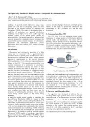
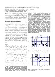
Figure 1 Left figure: Total column ozone values measured at KLI, Arosa by 

Brewer spectrophotometer #040. Right figure: Aerosol optical depth 

measurements at 368 nm from a Precision Filter radiometer at PMOD/WRC 

The total column ozone is shown in the left graph of Figure 1 and was 

obtained from Brewer spectrophotometer #040 located at the Licht- 

Klimatisches Observatorium in Arosa, about 20 km horizontal distance from 

Davos at an altitude of 1800 m.a.s.l. The total column ozone varied between 

293 and 362 DU with a mean value of 322 DU over the measurement period. 

The aerosol optical depth (aod) at 368 nm, measured with PFR 

sunphotometers is shown in the right graph of Figure 1; the aod was between 

0.05 and 0.1 on the clear sky days of August 15, 18 and 23. The afternoon of 

15 August was perturbed by cirrus clouds. 

3. Instrumentation 

Thirty-six radiometers measuring erythemally weighted solar irradiance from 

31 Institutions of 16 Countries took part in this campaign. A list of the 

participating radiometers is shown in Table 1. As can be seen from the table, 

the radiometers represented the most widely used instruments used for the 

measurement of erythemal weighted solar irradiance, namely 18 SL-501 

radiometers from Solar Light Inc., 9 UVB-1 radiometer of Yankee 

Environmental Systems, Inc., and 7 radiometers from Scintec or Kipp&Zonen. 

One Eldonet radiometer and one SRMS system based on a SL-501 

radiometer also participated at the campaign. 

The analog voltages of the radiometers were acquired with an Agilent 34970A 

multiplexer unit with 60 channels and a repeat rate of 6 seconds. The Eldonet 

and SRSM systems used their own data acquisition system and stored 

measurements as one minute averages. The digital SL-501 radiometers were 

set to acquire one minute averages, and when possible their sensitivity factor 

was set to 10 to improve their resolution. 

7

Table 1 List of participating radiometers 

Country Instrument Manufacturer Institution ID 

Spain UVB-1 941204 YES 

the 

Netherlands 

SL-501 5782 

UVB-1 030521 

UVB-1 990608 

UVB-1 970839 

K&Z 000518 

Sweden SL-501 0922 

Solar Light, 

Analog 

YES 

YES 

YES 

Kipp & Zonen 

Instituto Nacional de Meteorología de 

España, Madrid (INM) 

MeteoGalicia, Santiago de Compostela (A 

Coruña), Spain 

Departamento de Física Aplicada, 

Univeristy of Granada, Spain 

Instituto Nacional de Técnica Aerospacial – 

INTA, Huelva, Spain 

Izaña Atmospheric Observatory, INM, 

Spain 

Universidad de Extremadura, Badajoz, 

Spain 

BB01 

BB20 

BB24 

BB29 

BB31 

BB30 

UV-S-E-T 20599 Kipp & Zonen Kipp & Zonen B.V., the Netherlands BB02 

SL-501 8885 

Solar Light, 

Digital 

Solar Light, 

Analog 

U.S. UVB-1 000904 YES 

France UVB-1 920906 YES 

Finland SL-501 635 

Switzerland SL-501 8891 

SL-501 1903 

SL-501 1904 

SL-501 1497 

SL-501 1492 

SL-501 1493 

Italy SL-501 5790 

UVB-1 030528 

Norway SL-501 1450 

Solar Light, 

Digital 

Solar Light, 

Analog 

Solar Light, 

Analog 

Solar Light, 

Analog 

Solar Light, 

Analog 

Solar Light, 

Analog 

Solar Light, 

Analog 

Solar Light, 

Analog 

YES 

Sveriges meteorologiska och hydrologiska 

institut (SMHI), Sweden 

Abisko Scientific Research Station, 

Sweden 

Central UV Calibration Facility (CUCF), 

NOAA, US 

Université des Sciences et Technologies 

de Lille, France 

Non-Ionizing Radiation Laboratory, STUK, 

Finland 

Federal Office of Meteorology and 

Climatology Meteoswiss, Switzerland 







PMOD/WRC 


National Research Council, Sesto 

Fiorentino 

Agenzia Regionale per la Protezione 

dell'Ambiente della Valle d'Aosta (ARPA 

Aosta) 

BB03 

BB07 

BB04 

BB05 

BB06 

BB08 

BB09 

BB10 

BB36 

BB17 

BB18 

BB11 

BB15 

UVB-1 970827 YES University of Rome ''La Sapienza'' BB26 

SL-501 0616 

Solar Light, 

Digital 

Solar Light, 

Digital 

U.K. K&Z 020614 Kipp & Zonen 

Norwegian Polar Institute, Norway 

Norwegian Radiation Protection Authority, 

Norway 

School of Earth Atmospheric and 

Environmental Sciences, University of 

Manchester 

BB12 

BB21 

BB13 

8

SRMS 26 

Custom 

Germany Eldonet XP Eldonet 

010-A-00360 

010-A-00407 

SL-501 4818 

Poland SL-501 0935 

K&Z 030616 

Slovakia SL-501 4811 

SL-501 5774 

Hungary SL-501 10403 

Scintec 

Scintec 

Solar Light, 

Digital 

Solar Light, 

Digital 

Kipp & Zonen 

Solar Light, 

Digital 

Solar Light, 

Analog 

Solar Light, 

Digital 

Greece UVB-1 921116 YES 

Austria 010-A-00349 Scintec 

Radiation Protection Division,Health 

Protection Agency, UK 

Friedrich-Alexander Universität, Institut für 

Biologie, Germany 

Deutscher Wetterdienst, Richard-Assmann- 

Observatorium Lindenberg 

Meteorologisches Institut der Universität 

München, Germany 

Institut für Meteorologie und Klimatologie 

(IMUK), University of Hannover, Germany 

Institute of Meteorology and Water 

Management, Legionowo, Poland 

Institute of Geophysics, Polish Academy of 

Sciences, Warsaw, Poland 

Slovak Hydro-meteorological Institute, 

Poprad, Slovakia 

Meteorological Observatory of the 

Geophysical Institute, Slovakia 

Hungarian Meteorological Service, 

Budapest, Hungary 

Laboratory of Atmospheric Physics, 

Aristotle University of Thessaloniki, Greece 

Division for Biomedical Physics, Innsbruck 

Medical University, Austria 

BB25 

BB14 

BB16 

BB28 

BB33 

BB19 

BB27 

BB22 

BB23 

BB32 

BB34 

BB35 

The traveling reference spectroradiometer QASUME provided the reference 

for the outdoor measurements; a second spectroradiometer from the Medical 

University of Innsbruck (UIIMP) participated at the outdoor measurements as 

secondary reference and backup solution in case of problems with the 

primary reference. In addition the presence of two spectroradiometers also 

allowed to ascertain the stability of the spectral solar irradiance 

measurements, as will be shown later. Both spectroradiometers were 

synchronised and measured solar irradiance spectra in the range 290 to 

400 nm every 15 minutes. 

4. Laboratory Characterisation 

The UV Laboratory at PMOD/WRC is essentially composed of infrastructure 

previously at the European Reference Centre for UV radiation measurements 

(ECUV) at the JRC Ispra, Italy which was moved and set-up at PMOD/WRC 

in 2005 [3]. 

The radiometers were turned on and temperature stabilised for at least one 

hour prior to their laboratory characterisation. Before the measurement, the 

dark signal and the temperature were monitored for five to ten minutes in 

order to check the default operating parameters (dark signal and temperature) 

of the radiometer. The characterisation itself was done without temperature 

stabilisation since cross-talk on the signal and power lines increased the 

observed variability of the measured signal. 

9

4.1 Relative spectral response Facility 

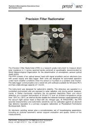
The relative spectral response facility is described in Hülsen and Gröbner [3]. 

It consists of a Bentham double monochromator DM-150 with gratings of 

2400 lines/mm. The wavelength can be selected within the range 250 to 500 

nm and the slit width was chosen to yield a nearly triangular slit function with 

a full width at half maximum of 1.9 nm. A 300 W Xenon lamp positioned in 

front of the entrance slit acted as radiation source and was adjusted so as to 

maximise the radiation at the exit slit. Behind the exit slit a quartz plate 

mounted at 45° relative to the vertical transmitted about 92% of the radiation 

towards the test detector while about 8% were deflected towards a 

photodiode which was used to check the stability of the monochromator 

signal. An iris with a diameter of 6 mm was placed in the beam path in front of 

the test detector to define the beam spot size. Due to the large receiving 

surfaces of the radiometers only part of the detector could be illuminated by 

the monochromatic light source. Thus, spatial inhomogeneities of the 

receiving surface of the radiometer were not taken into account during the 

spectral response function (SRF) measurement. The relative spectral 

throughput of the monochromatic light source (MLS) was determined by 

measuring the spectral response of the MLS with the QASUME 

spectroradiometer between 260 and 400 nm, every 5 nm. Between 380 and 

410 nm the rapidly changing spectral throughput of the MLS necessitated a 

step size of 1 and 2 nm. The wavelength scale of the MLS was determined by 

two methods which produced equivalent results: 

• A mercury discharge lamp was placed at the entrance of the 

monochromator and the throughput measured with a photodiode to 

determine the slit function and thus the wavelength offset. 

• The slit function measurements of the complete MLS (with Xe-Lamp 

source) with the QASUME spectroradiometer also allowed the 

determination of the wavelength offset from the slit function 

measurements. 

The wavelength scale over the range 250 to 400 nm could be determined by 

both methods to within ±0.1 nm. 

The variability of the dark signal was monitored for five minutes prior to the 

SRF measurement as indicator for the minimum signal to noise ratio of the 

radiometer. The SRF measurement itself was obtained over the wavelength 

range 260 to 400 nm with a step size of 2 nm; the whole measurement 

required about 10 minutes. The overall relative expanded uncertainty of 

measurement (k=2) of the SRF is estimated to be better than 10% for SRF 

values larger than 5·10 -4 . Lower values have an estimated uncertainty of 30% 

due to the larger measurement variability. 

The data-logger of the digital SL-501 radiometers were set to a sensitivity of 

10 to increase the resolution of the stored measurement. To further increase 

the signal to noise, the output signal was sampled 10 times at each 

wavelength setting of the monochromatic light source. This increased the 

measurement time relative to the analog radiometers to about 30 minutes. 

The SRF of the Eldonet radiometer could not be determined since the 

individual readings of the radiometer could not be accessed and synchronised 

with the wavelength setting of the MLS. 

The SRF was obtained from the measurements by subtracting the dark signal 

measured before initiating the wavelength scan, and normalising it to the 

maximum signal. 

10

4.2 Angular response Facility 

The angular response function (ARF) of the radiometer was measured on a 3 

m long optical bench. A 1000 W Xenon lamp was mounted at one end of the 

optical bench and served as radiation source. The detector was mounted on a 

goniometer at the other end with the vertical rotation axis passing through the 

plane of the receiving surface of the radiometer. The resolution of the rotation 

stage was 29642 steps per degree, or 0.12 arcseconds. The homogeneity of 

the radiation at the detector reference plane was measured and optimised to 

better than 1% over the receiving surface area of the detector. A baffle was 

placed in the beam path to reduce stray light within the dark room and a 

WG305 filter with a 50% cut off at 303 nm removed radiation below approx 

300 nm. A mirror glued onto the rotation stage reflected some of radiation 

back on the Xe-lamp source which provided an adjustment precision of better 

than 0.1 degree. The expanded relative uncertainty (k=2) of measurement is 

estimated to be less than 4% for zenith angles below 80%. 

The measurements were performed in two orientations of the detector so that 

the angular response could be determined for the four quadrants N, S, E, W, 

with the N orientation defined by the connector of the radiometer. 

The ARF of the Eldonet and the SRMS systems could not be measured 

because they could not be fitted on the goniometer. 

The ARF for each quadrant was obtained by normalising the measurements 

at each angle to the reference measurement at normal incidence. The cosine 

error of each quadrant was calculated from the ARF by assuming an isotropic 

radiation distribution and integrating it over the whole hemisphere. The final 

ARF was obtained by averaging the measurements of the four quadrants. 

4.3 Absolute Calibration 

The absolute calibration was obtained by a comparison of solar UV radiation 

measured with the radiometer and the co-located QASUME 

spectroradiometer. The irradiance spectra were weighted with the detector 

spectral response to produce the absolute calibration factor for each 

radiometer. The conversion function f (see right side of Figure 2) to convert 

from detector weighted solar irradiance to erythemal weighted irradiance was 

calculated with the following equation, 

∫CIE( 

λ)E 

f (SZA,TO3) 

= 

∫SRF( 

λ)E 

rad 

rad 

( λ)dλ 

( λ)dλ 

where E rad is a solar irradiance spectrum calculated with a radiative transfer 

model in dependence on solar zenith angle (SZA) and total column ozone 

TO 3 ; SRF(λ) and CIE(λ) represent the detector and erythemal spectral 

responses respectively (see left side of Figure 2). 

11

Figure 2 Left figure: radiometer spectral response function (red) and CIE- 

Erythema (blue). Right Figure: Conversion function f n (SZA,TO 3 ) to convert from 

detector weighted to erythemally weighted solar irradiance. 

For radiometers with a significant deviation of the angular response from the 

nominal cosine response, a cosine correction function has to be applied to the 

measurements. This correction depends on the atmospheric conditions and 

especially on the fraction of direct and diffuse radiation. The cosine correction 

applied for the data measured during the campaign used an isotropic diffuse 

radiation distribution; the fraction of direct and diffuse radiation was modeled 

by a radiative transfer model in dependence of the solar zenith angle (see 

Figure 3). For the determination of the calibration factor only two cases were 

distinguished: 

1. clear sky: A cosine correction function 1/f glo (SZA) in dependence on 

the SZA was used. 

2. diffuse sky: Only the diffuse cosine correction factor 1/f dif was applied 

to the calibration. 

Depending on the radiometer type this simple approximation resulted in 

substantial variabilities especially during rapidly changing cloud conditions. In 

these cases, only the clear sky days were used for the calibration. 

f dir 

ARF( θ) 

= 

cos( θ ) 

f 

dif 

pi 

2 

= 2 ⋅ ∫0 

ARF( θ) sin( θ) 

dθ 

E 

E 

dir 

f 

glo 

= f 

dir 

+ 

glo 

f 

dif 

E 

E 

dif 

glo 

Figure 3 Angular response function of a YES radiometer (circles) and the 

nominal cosine response function (blue curve). 

f dir is the cosine error of the radiometer, f dif represents the diffuse cosine error 

and f glo the global cosine error of the radiometer. The radiometer shown in 

Figure 3 has a diffuse cosine error of 0.84, i.e. it underestimates the diffuse 

irradiance by 19%. 

12

4.4 Horizon at PMOD/WRC 

The horizon of the measuring site is limited by the surrounding mountains, as 

can be seen in Figure 4. The horizon actually obstructed the sun for SZA 

above 70º. For an isotropic diffuse radiation distribution the horizon would 

block about 5% of the total diffuse radiation. 

Figure 4 Horizon as observed from the roof platform of PMOD/WRC. North is 

Azimuth 0 and South is Azimuth 180. 

We have estimated the effect of this horizon on the radiometers, taking into 

account their different angular responses. The resulting diffuse cosine error 

for each radiometer was calculated for either a full hemisphere or one with the 

horizon of PMOD/WRC. 

Figure 5 Relative deviation between the cosine error determined for a full 

hemisphere to the one of the PMOD/WRC horizon determined for each 

radiometer. The largest deviations are between +0.4% and -0.8%. 

Figure 5 shows the ratio between these two values which represents the error 

made if a diffuse cosine correction is applied without taking into account the 

real horizon of the measurement site. As can be seen in the figure, the largest 

influence is of the order of 0.8% for a total overcast sky and even less for a 

clear sky where this error would be reduced by the direct to diffuse radiation 

13

atio. The calibrations at PMOD/WRC were calculated using the diffuse 

cosine correction factor calculated for the PMOD/WRC horizon. 

4.5 The effect of a finite scan time 

The two spectroradiometers measured solar irradiance spectra by moving the 

diffraction gratings and measuring each wavelength sequentially. This 

resulted in a typical scan time of about 8 minutes for the wavelength range 

290 to 400 nm. The following procedure was used to take into account the 

changing conditions during each scan, such as changing solar zenith angle or 

cloud variabilities: 

Figure 6 Solar spectrum measured with the QASUME spectroradiometer (blue 

curve), radiometer spectral response function (green curve), and detector 

weighted spectral irradiance (black curve). The red circles represent the 

radiometer readings during the scan time of the spectroradiometer. 

At the core of the method is the availability of a large number of individual 

radiometer readings U(t) during a single solar spectrum measurement (see 

Figure 6). The solar spectrum, as measured by the spectroradiometer, is 

weighted with the detector spectral response to produce a spectral detectorweighted 

solar irradiance E DET (λ) 

E DET 

( λ ) = SRF( λ) 

⋅E( 

λ) 

The detector weighted solar irradiance E DET is further obtained by integrating 

E DET (λ) over the whole wavelength interval and the representative time T DET 

by integrating the weighted time of the solar spectrum with E DET (λ) 

E 

T 

U 

DET 

DET 

DET 

= 

= 

= 

∫ 

∫ 

∫ 

E 

DET 

( λ)dλ = 

SRF( λ)E( 

λ)t 

( λ)dλ 

/ E 

∫ 

SRF( λ)E( 

λ)U(t 

I 

SRF( λ)E( 

λ)dλ 

I( λ) 

DET 

)dλ 

/ E 

DET 

14

This effectively means that the radiation contribution of each wavelength 

weighted with the detector sensitivity is used as measure for the “relative 

importance” of each wavelength to the total measured irradiance. The 

radiometer readings during the time of the solar spectrum scan were 

weighted with E DET (λ) to produce an average radiometer signal for each solar 

irradiance scan. 

4.6 The complete radiometer calibration equation 

The calibration procedure used during this campaign to transform raw signals 

from a radiometer to erythemally weighted solar irradiance is based on the 

following equation: 

E = (U − U ) ⋅C⋅f 

(SZA,TO ) ⋅Coscor 

CIE 

offset 

n 

3 

where E CIE is the erythemal effective irradiance, U is the measured electrical 

signal from the radiometer and U offset is the electrical offset for dark conditions 

[4, 5]. C is the calibration coefficient, determined for a SZA of 40° and total 

column ozone of 300 DU. f n (SZA, TO 3 ) is a function of SZA and total column 

ozone (TO 3 ) to convert from detector based to erythemal based effective 

irradiance. By definition the function is normalised to unity for a total ozone 

column of 300 DU and a solar zenith angle of 40°. Coscor represents a 

cosine correction function which uses the ARF determined in the laboratory. 

The dark offset U offset was determined every day of the campaign during the 

night as the average over all measurements between 0 to 4 UT and 20 to 24 

UT. The Cosine correction Coscor was calculated following the procedure 

described before and applied to the raw measurements U. 

The calibration coefficient C at the time T DET was then obtained by 

comparison with the solar spectrum measured by the spectroradiometer 

weighted with the SRF of the radiometer. Thus, 

C = 

U 

DET 

E 

DET 

− U 

offset 

⋅ 

1 

Coscor 

1 

⋅ 

f (40°,300DU) 

5. Campaign Results 

5.1 Spectroradiometer intercomparison 

The reference spectroradiometer QASUME and the DM-300 

spectroradiometer from the Medical University of Innsbruck measured 

synchronised solar irradiance spectra in the range 290 to 400 nm every 0.25 

nm every 15 minutes. The instrument entrance optics were located within less 

than 50 cm from each other at the same height. Before installing the 

instruments on the roof, each spectroradiometer was calibrated with its own 

reference standard (portable lamps). Two of these lamps were also measured 

by the spectroradiometer of the other institute to determine the difference 

between the absolute reference of the respective laboratories. These 

measurements are shown in Figure 7 and demonstrate that the irradiance 

reference of the Medical University of Innsbruck is about 1% lower than the 

QASUME reference. This observed difference was not taken into account in 

the later analysis. 

15

Figure 7 Comparison of two irradiance standards (portable lamps) of the 

Medical University of Innsbruck (K5) and of PMOD/WRC (T68524), measured 

respectively by the other institute. 

The comparison of the solar irradiance spectra followed the standard 

operating procedure of a QASUME intercomparison, i.e. the spectra were 

convolved to a 1 nm slit width and wavelength adjusted to a common 

wavelength scale. The comparison of all measurements at selected 

wavelengths and the average over the measurement period is shown in 

Figure 8 . 

Figure 8 Comparison of spectral solar irradiance measurements between UIIMP 

and QASUME. The left figure shows the comparison over the whole 

measurement period for selected wavelength bands. The right figure shows the 

average spectral ratio between UIIMP and QASUME. The 90% variability is 

indicated by the two gray lines. 

As can be seen in the figure the average difference between the two 

instruments is 0% with a variability of less than or equal to 2% for 90% of all 

measured spectra (658 out of 731). The observed diurnal variation was also 

below 2% for most days. For the clear sky days the diurnal variation was of 

the order of 5%; the pattern of this diurnal variation could be traced to an 

azimuth dependence of the angular response of the entrance optic used by 

UIIMP. This azimuth dependence was identified on August 23 by rotating the 

entrance optic of UIIMP by 180º and observing the expected change of 2 to 

3% in the spectral ratio relative to the QASUME spectroradiometer, which 

was left unchanged. 

16

5.2 Radiometer Absolute Calibration 

a 

b 

c 

Figure 9 Calibration factors determined for the campaign period for three 

sample radiometers representing the threre main types of radiometers present 

at the intercomparison, drawn against SZA; Figure 4a: YES (BB01), Figure 4b: 

SL-501 (BB17), and Figure 4c: Scintec (BB16). The plots actually show the 

inverse of C as defined in the equation above to facilitate the interpretation. A 

lower calibration factor means a lower signal measured with the radiometer. 

The green curves represent the cosine corrections calculated for each 

radiometer based on the ARF measured in the laboratory. 

Figure 9a, 9b and 9c show the calibration coefficients of three sample 

radiometers from YES (BB01), Solar Light (BB17), and Scintec (BB16), for 

the whole campaign computed with the procedure described in the preceding 

paragraph but without applying the cosine correction to the calibration factor 

C. The cosine correction was added as a separate function (green curve) and 

normalised to one at 40 SZA. A clear sky cosine correction (function with 

SZA) was only applied on the clear sky days (15, 18, and 23 August); all other 

17

days used a diffuse cosine correction (constant factor). For days with rapidly 

changing cloud conditions such as August 19 (day of year 231) for example, 

the increased variability of the calibration factor for instruments with a large 

cosine correction is apparent. This variability is explained with the inadequate 

cosine correction for these atmospheric conditions. These graphs also 

demonstrate that the observed diurnal variability of the calibration factor for 

the clear sky days can be almost completely explained with the cosine 

correction, i.e. the deviations of the ARF from the nominal cosine function. 

The cosine corrections for the three main types of radiometers in this 

campaign were: 

• less than 3% for Kipp & Zonen or Scintec radiometers 

• between 6% to 15% for Solar Light SL-501 radiometers 

• between 14% and 25% for YES UVB-1 radiometers. 

The expanded uncertainty of measurement (k=2) of the calibration for all 

radiometers were of the order of 7%. The largest contribution came from the 

uncertainty of the reference spectroradiometer of about 5%. The variability of 

the radiometers during the calibration contributed only the remaining 2% of 

this uncertainty. Some instruments showed a higher variability which resulted 

in a larger uncertainty. The individual characterisation and calibration results 

for each radiometer are summarised in Table 2 and graphs are shown in the 

Annex. Two instruments were unstable during the campaign: The calibration 

factor determined for BB02 showed large diurnal variations which could be 

traced to a significant change in the spectral response of the instrument 

between the first measurement on August 1 and the second measurement on 

24 August after the campaign. The Eldonet radiometer showed unexplained 

variations of about 10% during the measurement campaign, with even larger 

deviations of 60% on the morning of August 15. 

6. Radiometer comparison 

The comparison of broadband UV radiometers allows two types of analyses. 

In the first type, the results of the broadband radiometers are compared with 

the results of the spectroradiometer (the QASUME reference). In this case, 

the UV indices derived from the broadband radiometer measurements are 

compared with UV indices derived from QASUME. Such an analysis allows 

verifying how well the reference results can be reproduced with the 

broadband radiometers, i.e., it allows empirically estimating the uncertainty of 

the calibration procedure. 

In the second type of analysis, the broadband UV radiometers are compared 

to each other. Since the goal in this case is to estimate the short-term 

statistical random uncertainty, the broadband radiometers are not anymore 

compared to QASUME, because of its longer integration time. 

6.1 Comparison of broadband radiometer with the reference 

spectroradiometer QASUME 

UV indices derived from the broadband UV radiometers were compared to 

concurrent UV indices derived from the reference QASUME 

spectroradiometers. The reference UV indices from the reference 

18

spectroradiometer QASUME were derived by integrating each solar spectrum 

by the CIE action spectrum and calculating the reference time of the 

calculated UV index by weighting the time stamp at each wavelength with the 

CIE-weighted irradiance at this wavelength and integrating over all time 

stamps of the spectrum (see description in section 4.5). 

Figure 10 Average relative differences between the radiometers and the 

QASUME reference spectroradiometer for the two solar zenith angle 

ranges 1) smaller than 50° and 2) higher than 65° and lower than 75°. 

Two sets of UV indices from the broadband radiometers were compared to 

the reference. For the first set, the raw signal measured by the radiometers 

during the campaign were communicated to the instrument owners who were 

asked to derived UV indices applying the procedures and calibration values 

they used prior to the campaign (thereafter described as prior (or owner) 

calibration). For the second set, UV indices were derived by PMOD/WRC 

using procedures and calibration values determined during the campaign 

(thereafter described as campaign calibration). The comparison between the 

UV indices derived for each radiometer and the QASUME spectroradiometer 

are shown in the Annex for each instrument. In addition the average relative 

differences between each radiometer and the QASUME reference for two 

SZA ranges (SZA below 50º and for SZA between 65º and 75º) are listed in 

Table 2 and shown in Figure 10. 

19

Table 2 Summary of the calibration performed at the PMOD/WRC-COST726 

calibration and intercomparison campaign of broadband radiometers 

measuring erythemally weighted solar irradiance, 28 July to 23 August 2006. 

The fifth column shows the relative difference in UV indices calculated by the 

instrument owners using their home calibration relative to the QASUME derived 

UV indices for low and high SZA ranges. 

Radiometer 

type 

Serial 

Number 

Days used for the 

calibration (August 06) 

Calibration Factor at 

40º and 300 DU 

Ratio E ERY, 

Owner calib. 

to QASUME 

SZA 

ID 

970827 15,18,23 0.1104 W m -2 nm -1 V -1 0.97 1.02 BB26 

990608 15,18,23 0.1199 W m -2 nm -1 V -1 0.99 0.93 BB29 

970839 15,18,23 0.1178 W m -2 nm -1 V -1 0.86 0.90 BB31 

921116 15,18,23 0.1506 W m -2 nm -1 V -1 0.99 0.97 BB34 

Scintec 

010-A 

00360 9-11,13,15,18,22-23 0.2143 W m -2 nm -1 V -1 1.42 1.64 BB16 

00407 9-11,13,15,18,22-23 0.1295 W m -2 nm -1 V -1 1.05 1.11 BB28 

00349 9-11,13,15,18 0.1474 W m -2 nm -1 V -1 1.03 1.02 BB35 

Kipp & 

Zonen 

020599 9-11,13,15,18,22-23 N/A unstable inst. 0.95 0.85 BB02 

020614 10,11,13,15,18,22-23 0.1113 W m -2 nm -1 V -1 0.84 0.40 BB13 

030616 10,11,13,15,18,23 0.2339 W m -2 nm -1 V -1 0.77 0.92 BB27 

000518 9-11,13,15,18,22-23 0.1062 W m -2 nm -1 V -1 1.09 1.15 BB30 

Eldonet XP 084 10-13,15 N/A unstable inst. 0.27 0.43 BB14 

21

6.2 Comparisons using Taylor diagrams. 

The broadband and spectroradiometer measurements were performed at 

different frequencies. The spectroradiometer needed an integration time of 

about 8 min. Most of the broadband radiometers were measuring with time 

steps of about 7 sec, but some of them, typically the SolarLight radiometers 

with digital read-out, measured at 1 Hz, but only recorded the 1-min average. 

In order to accommodate all different repeat rates, times were defined for 

each QASUME measurement by using a weighted average, then a two 

minute window was defined around each of these time points (QASUME 

measurement time ± 1 min). Finally, for each broadband radiometer bbXX, 

QASUME-concurrent UV indices were determined by averaging the bbXX UV 

indices in each two minute window. For each bbXX, this procedure was 

repeated for UV indices determined using the prior and the campaign 

calibration, leading to two time series of QASUME concurrent UV indices for 

each bbXX (see Figure 11). 

The agreement between UV indices determined by the QASUME reference 

and by the broadband UV radiometer (bbXX) is evaluated using Taylor 

diagrams ([6], see Appendix). In addition, each comparison was carried out 

using two time selections. In the first selection, all times when the solar zenith 

angle was less than 70º were selected, and in the second selection an 

additional criterion was used based on the smoothness of the UV index as a 

function of cosine solar zenith angle in order to select clear-sky times. Figure 

11 (right panel) shows the data that satisfy only the solar zenith angle 

criterion in red and data satisfying both criteria in blue. Thereafter, the data 

set including all times with solar zenith angle less than 70º will be referred as 

all-sky, while the subset satisfying the additional criterion will be referred as 

clear-sky. In addition, a further subdivision was introduced for the analysis 

between times when the solar elevation was low (solar zenith angle between 

50 and 70º) and times when the solar elevation was high (solar zenith angle 

between 30 and 50º, the minimum solar zenith angle reachable during the 

inter-comparison was slightly higher than 30º). 

22

Figure 11 UV indices measured during the inter-comparison. Left top panel: UV 

indices measured by the QASUME reference and the broadband UV erythemal 

radiometer YES UVB-1 000904 (bb04). The red curve is the QASUME 

measurement, the blue curve is the bb04 determination using the prior 

calibration, and the green curve is the bb04 determination using the campaign 

calibration. Left down panel: Ratio between the bb04 UV index using prior 

calibration and using campaign calibration (red curve), and ratio between bb04 

UV index (campaign calibration) and QASUME UV index. Right panel: UV 

indices of times selected for the comparison between broadband radiometers 

and the QASUME reference. Times satisfying the UV index vs. cosine solar 

zenith angle smoothness criterion are shown in blue (clear-sky), and times not 

satisfying this criterion are shown in red. 

Taylor diagrams summarising the agreement of the UV indices measured by 

the broadband radiometers with the UV indices measured by the QASUME 

reference are shown in Figure 12. On the panels on the left, the agreement is 

evaluated using times for all sky with different selections on the solar zenith 

angle, while the panels on the right use only times corresponding to the clearsky 

selection. The panels on the first row show the comparison using all solar 

zenith angles below the 70º limit, the second row corresponds to solar zenith 

angles below 50º (high solar elevation), while the third row corresponds to 

solar zenith angles between 50 and 70º (low solar elevation). On all panels, 

the crosses correspond to the UV indices determined with the prior 

calibration, while the dots correspond to the campaign calibration. The black 

cross on the horizontal axis corresponds to the reference. 

Because the different diagrams apply to different data sets with a relatively 

wide range of standard deviation (the standard deviation of the reference data 

set is shown by the position of the black cross on the horizontal axis), the 

Taylor diagrams are given in absolute unit (UVI), rather than relatively to the 

standard deviation of the reference. For example, the black cross on panel (a) 

shows that the standard deviation of the whole reference UVI data set is 

about 1.75 (all-sky and all solar zenith angles below 70º). Data points at the 

same radius than the reference indicate that the UVI data set measured by 

the corresponding radiometer has a standard deviation equal to the data set 

measured by the reference, and consequently gives the same result than the 

reference in average. The angle between the radius to the data point and the 

horizontal axis indicate how well the data set of the corresponding radiometer 

is correlated with the reference data set. The distance between the black 

cross and the data points indicates the centered RMSE between the data set 

of the corresponding radiometer and the reference data set in UVI units. 

Finally, the orientation of the segment between the data points and the black 

cross indicates whether the RMSE is mainly due to a bad normalisation 

(segment almost parallel to the horizontal axes, corresponding to high 

23

correlation) or to a lack of correlation (segment close to the perpendicular to 

the horizontal axes). 

Figure 12 Taylor comparison of broadband radiometer-measured UV indices 

with UV indices measured by the QASUME reference. The crosses illustrate the 

agreement with the reference when using the original calibration from the 

instrument owner and the dots show the agreement when using the 

calibrations determined during the inter-comparison. The different panels show 

the comparisons for different selections based on solar zenith angles and clear 

sky times or all-sky times (both clear-sky and cloudy-sky times – see figure 11). 

Panel a) all-sky, SZA 30 to 70º, 

b) clear-sky, SZA 30 to 70º, 

c) all-sky, SZA 30 to 50º, 

d) clear-sky, SZA 30 to 50º, 

e) all-sky, SZA 50 to 70º, 

f) clear-sky, SZA 50 to 70º. 

In all cases, Taylor diagrams demonstrate a high correlation between 

broadband radiometers and the QASUME UV indices. It is only when 

comparing data for all-sky times at high solar elevation (panel c), that one 

instrument is shown to have a correlation below 0.98. On the other hand 

when comparing clear-sky UV indices for all solar zenith angles (panel b), the 

correlation is higher than 99.8% for all instruments. Such a high correlation is 

expected because the variations of UV indices are mostly driven by external 

factors such as solar zenith angle or cloudiness to which all the broadband 

radiometers respond similarly, whether they are correctly calibrated or not. 

Consequently, very large RMSE between the reference and the broadband 

radiometers are only found for some instruments, when using prior 

24

calibration, and in case of large normalisation error. In such case, the 

influence of the correlation is negligible. For a few instruments, normalisation 

errors larger than 25% are found. 

Comparisons using all-sky situations are more difficult to interpret. In such 

situations lower correlations can be due to a multiplicity of factors. In some 

cases, differences in measurement frequency can play a role, because rapid 

changes occur for broken cloud coverage. Correlation for instruments having 

large cosine correction can also suffer from the fact that the cosine error was 

applied only for clearly identified clear-sky situations. In case of broken cloud 

with direct sunshine on the instrument, the direct beam cosine correction 

should also be applied, but was not. However, the instrument showing the 

most important lack of correlation in panels a, c and e is a Scintec radiometer 

when applying prior calibration. Thus, the effect of cosine error should 

probably be ruled out in this case. The clearest pattern for all-sky cases is 

that SL501 radiometers with digital readout and, to a lesser degree, SL501 

radiometers with analog readout seem to group in clusters with nearly 

identical correlation with the reference. Instruments in each group (SL501D 

and SL501A) measured with a particular frequency pattern. SL501D 

radiometers used 1Hz measurement frequency and recorded 1-min averages, 

while SL501A measured about every 7s and recorded all measurements. 

(Except one SL501A that used a measurement frequency similar to the 

SL501D). Thus, the observed pattern for SL501D, and to a lesser degree for 

SL501A, may be due to difference in measurement frequency between the 

broadband radiometers and the spectro-radiometer. 

In clear-sky cases, panel b of Figure 12 shows that most instruments have an 

RMSE with the reference of less than 0.25 UVI (the first equal-RMSE circle is 

at 0.5 UVI), with a very high correlation. As mentioned earlier this high 

correlation reflects only a similar response to external factors. Restricting the 

analysis to a given solar zenith angle domain allows diminishing the influence 

of such external factors, especially for clear-sky cases since the solar 

elevation is then the dominant factor. Panel d shows that when restricting to 

high solar elevation, the RMSE does not diminish as much as the standard 

deviation of the reference data set: Most instruments have an RMSE of less 

than 0.2 (first equal-RMSE circle is at 0.2 UVI), but the standard deviation of 

the reference data diminishes from about 2 UVI when considering all solar 

zenith angles to slightly less than 1.2 when considering only high solar 

elevation. In this case, for many instruments, the rcorrelation with the 

reference is reduced and contributes significantly to the RMSE, when the 

analysis is restricted to high solar zenith angles. When restricting to low solar 

elevation, most instruments have an RMSE below 0.1, while the reference 

data set standard deviation is about 0.8. Here, the correlation is high (similar 

to considering all solar zenith angle) and not contributing much to the RMSE. 

The difference in the influence of correlation on the RMSE between high and 

low solar elevation data set can be explained by the fact that solar elevation 

influence UV radiation proportionally to the air mass, which changes much 

more rapidly at low than at high solar elevation. Thus, this external 

dominating factor has more influence for the low solar elevation data set, 

which leads to higher correlation. 

In Figure 12, the agreement between the UV indices measured by the 

broadband radiometers and the reference are illustrated for both prior and 

campaign calibration. A light dotted line joins the cross to the dot for each 

instrument. The new calibration brings an improvement when the dot is closer 

to the reference point (black cross). Both for clear-sky cases and all-sky 

cases most instruments show a marked improvement, and for some 

25

instruments there is no significant change. For clear-sky cases, the 

improvement is mainly occurring in the direction of better normalisation 

(overall calibration factor). However, when all-sky cases are considered, 

some instruments show a significant improvement in the correlation, which is 

likely to be due to a better consideration of zenith angle and ozone effects. 

Finally, considering only clear-sky cases and using the calibration determined 

during the intercomparison, the relative RMSE between the broadband 

radiometer and the QASUME reference is on the order of 0.1 UVI or less for 

all instruments when restricting to high solar elevation and even lower on the 

order of 0.04 UVI when restricting to low solar elevation (see Figure 13). This 

is better than 10% for high solar elevation and on the order of 5% for low 

solar elevation. This indicates that for clear-sky cases, broadband UV 

radiometers that are recently and properly calibrated can reproduce the 

reference measurements with an uncertainty of about 5–10%. This 

reproducibility was achieved for more than 30 instruments including all major 

manufacturers of such instruments. 

Figure 13 Taylor comparisons of broadband radiometer-measured UV indices 

with UV indices measured by the QASUME reference. Selected clear-sky cases 

and UV indices using PMOD/WRC calibrations. The inner circle indicates a 

centered RMSE of 0.1 UVI. Panel a) clear-sky, solar zenith angle 30 to 50º, b) 

clear-sky, solar zenith angle 50 to 70º. 

6.3 Instrument random (statistical) uncertainty 

The short-term random variability of the broadband UV radiometers was 

estimated by inter-comparing their measurements. Because of integration 

time issues, the QASUME was not chosen as reference. The average of all 

valid UV-indices measurements from all broadband UV radiometers for each 

two-minute window were taken as reference, under the assumption that shortterm 

statistical variability will cancel out between instruments 1 . For each 

instrument, the ratio of the average UV index to the UV index measured by 

the given instrument using campaign calibration is fitted with a quadratic 

response surface to empirically express systematic solar zenith angle and 

ozone dependences (see Figure 14) that would not have been captured by 

the campaign calibration procedure. 

1 Other combinations were tried such as all broadband radiometers except the 5 instruments 

with largest residuals to the average, or three instruments of each manufacturer having the 

smallest RMSE with the QASUME reference, but results were similar to results obtained with 

average of all instruments taken as reference. 

26

Figure 14 Ratio of average UV index to single instrument-measured UV index 

as a function of ozone total column and cosine solar zenith angle. The black 

dots are the individual measurement ratios, and the colored surface show the 

quadratic response surface fit. The left panel shows an example with small 

residuals, while the right panel shows an example with large residuals. 

This method is chosen for isolating the random uncertainty as much as 

possible, and not including the systematic effects that could be linked to the 

known influential parameters mentioned above. Thus, the residuals between 

the measurement ratios and the fit surface are analysed for estimating the 

random variability of the instruments. Similarly to the Taylor diagram analysis, 

this analysis was repeated considering first only cases considered as clearsky, 

then considering both clear- and cloudy-sky (see Figure 11). 

Analysis of the residuals in clear-sky cases shows that the random statistical 

variability is below ±2% (for many instruments, it is more of the order of ±1%). 

It also seem that most SolarLight radiometers with analog read-out (SL501 A) 

have a small random variability, while many SolarLight radiometers with 

digital read-out have larger than average random variability (see Figure 15). 

Analysis of residuals for all-sky cases shows much larger random variability, 

which is most likely due to quick variations of UV radiation level when partial 

cloud coverage is occurring. In all-sky cases, the short-term random variability 

is on the order or below ±5% (see Figure 16). As was the case in the clearsky 

analysis, SolarLight radiometers with analog read-out have smaller than 

average random variability. On the other hand, instruments with larger than 

average variability seem not to be of a specific type. As was the case in the 

Taylor diagram analysis, subsets including only solar zenith angles between 

30 and 50º, and between 50 and 70º were analysed separately. However, 

there were no significant differences in the analysis results when the subsets 

were analysed separately or together. 

27

SL01085 bb37 

SL01497 bb36 

SC00349 bb35 

YS921116 bb34 

SL04818 bb33 

SL10403 bb32 

YS970839 bb31 

KZ000518 bb30 

YS990608 bb29 

SC00407 bb28 

KZ030616 bb27 

YS970827 bb26 

SRMS26 bb25 

YS030521 bb24 

SL05774 bb23 

SL04811 bb22 

SL00616 bb21 

SL05782 bb20 

SL00935 bb19 

SL01493 bb18 

SL01492 bb17 

SC00360 bb16 

YS030528 bb15 

Eldonet bb14 

KZ020614 bb13 

SL01450 bb12 

SL05790 bb11 

SL01904 bb10 

SL01903 bb09 

SL08891 bb08 

SL08885 bb07 

SL00635 bb06 

YS920906 bb05 

YS000904 bb04 

SL00922 bb03 

KZ020599 bb02 

YS941204 bb01 

−0.02 −0.015 −0.01 −0.005 0 0.005 0.01 0.015 0.02 

Residuals 

SL501 A 

SL501 D 

YES 

K&Z + Sc 

Misc 

Figure 15 Distribution of residuals for selected clear-sky situations. Boxes 

represent the inter-quartile range of the distribution. The dashed lines show the 

extent of the rest of the distribution, except if there are outliers, that are defined 

as values that are more than 1.5 times the inter-quartile range away from the 

extremities of the boxes. In some cases large groups of outliers are present. It is 

due to the high auto-correlation of the data, which leads to clusters of outliers. 

SL01085 bb37 

SL01497 bb36 

SC00349 bb35 

YS921116 bb34 

SL04818 bb33 

SL10403 bb32 

YS970839 bb31 

KZ000518 bb30 

YS990608 bb29 

SC00407 bb28 

KZ030616 bb27 

YS970827 bb26 

SRMS26 bb25 

YS030521 bb24 

SL05774 bb23 

SL04811 bb22 

SL00616 bb21 

SL05782 bb20 

SL00935 bb19 

SL01493 bb18 

SL01492 bb17 

SC00360 bb16 

YS030528 bb15 

Eldonet bb14 

KZ020614 bb13 

SL01450 bb12 

SL05790 bb11 

SL01904 bb10 

SL01903 bb09 

SL08891 bb08 

SL08885 bb07 

SL00635 bb06 

YS920906 bb05 

YS000904 bb04 

SL00922 bb03 

KZ020599 bb02 

YS941204 bb01 

−0.1 −0.08 −0.06 −0.04 −0.02 0 0.02 0.04 0.06 0.08 0.1 

Residuals 

SL501 A 

SL501 D 

YES 

K&Z + Sc 

Misc 

Figure 16 Same as Figure 15, but for all-sky situations. (Note that the 

horizontal scale is 5 times larger than in Figure 15). 

28

Acknowledgments 

We would like to acknowledge the active support of the PMOD/WRC staff in 

the preparation and organisation of the intercomparison campaign. The 

instrument owners provided the calibrated data for the intercomparison period 

using their home calibration. The total ozone column measurements from 

Arosa were provided by Meteoswiss. The instrumentation of the UV 

Calibration Section of the PMOD/WRC is made available by the Joint 

Research Centre of the European Commission in Ispra under cooperation 

agreement 2004-SOCP-22187. G. Hülsen is supported by the Swiss COST 

Office under contract C05.0068. D. Walker is supported by the Swiss State 

Secretariat for Education and Research, COST Office, under contract 

C04.0242. Financial support of the stay of J.E. Gil from the Ministerio de 

Educación y Ciencia and FEDER funds from CGL2004-05984-C07-03, 

REN2003-03175 projects are gratefully acknowledged. The participation of M. 

Blumthaler and J. M. Vilaplana at the campaign was partly financed by COST 

726 (STSM-COST726-03 and STSM-COST726-04). 

. 

29

References 

[1] K. Leszczynski, K. Jokela, L. Ylianttila, R. Visuri and M. Blumthaler. 

Erythemally weighted radiometers in solar UV monitoring: Results from the 

WMO/STUK Intercomparison. Photochem. Photobiol., 67:212–221, 1998. 

[2 ]WMO/GAW Report No. 141: Report of the LAP/COST/WMO 

Intercomparison of Erythemal radiometers, Thessaloniki, Greece, 1999. 

WMO TD{No. 1051}. 

[3] Hülsen, G., and J. Gröbner, Characterisation and Calibration of UV 

Broadband radiometers Measuring Erythemally Weighted Irradiance, 

Applied Optics, 46, 5877-5886, 2007. 

[4] A. Webb, J. Gröbner, and M. Blumthaler. A Practical Guide to Operating 

Broadband Instruments Measuring ErythemallyWeighted Irradiance, 2007. 

EUR 22595, ISBN 92-898-0032-1. 

[5] G. Seckmeyer, A. F. Bais, G. Bernhard, M. Blumthaler, C. R. Booth, R.L. 

Lantz, R.L. McKenzie, P. Disterhoft, and A. Webb. Instruments to measure 

solar ultraviolet radiation. Part 2: Broadband Instruments Measuring 

Erythemally Weighted Solar Irradiance. WMO/GAW No. 164 World 

Meteorological Organization, Geneva, 2007. 

[6] Taylor, K. E. (2001), Summarizing multiple aspects of model performance 

in a single diagram, J. Geophys. Res., 106(D7), 7183–7192. 

30

Appendix: Taylor diagram comparison 

Taylor diagrams (Taylor, 2001) are a tool for evaluating the agreement 

between a tested data set and a reference data set (with one-to-one 

correspondence between the tested data points and the reference data 

points). The evaluation of the agreement between a given data set and the 

reference data set is illustrated by a single point on the Taylor diagram, which 

gives information about the relative normalisation between the tested and 

reference data set, their correlation and the root mean square error (RMSE) 

between the two sets. Since the information on the agreement of a given data 

set with the reference is given by a single point, many tested data sets can be 

compared to a single reference in a given Taylor diagram. 

Taylor diagrams are based on the recognition that the relative standard 

deviation (the ratio of the tested data set standard deviation over the 

reference data set standard deviation), the centered root mean square error 

(see Taylor, 2001 for definition), and the correlation can be seen as the 

different components of the law of cosines with the correlation being the 

cosine of the angle. 

Figure A-1 Example of comparison for synthetic data sets. Left panel: tested 

data sets shown together with the reference data set. Middle panel: tested 

data sets shown as function of the reference data set. Right panel: Taylor 

diagram comparison of tested data sets with reference. 

Figure A1 shows an example of Taylor diagram comparison between two 

synthetic tested data sets and a corresponding reference. On the left panel, 

the reference data set is shown in red, while the first tested data set has a 

different overall normalization (in blue), and the second has a phase shift (in 

green). On the middle panel, the two tested data sets are shown as function 

of the reference data set. The first data set has a good correlation with the 

reference data set, but the slope of the regression line is lower than 1. The 

second data set has a regression slope of 1, but a worse correlation than the 

other data set. The right panel shows the Taylor diagram comparison of the 

tested data sets with the reference. The Taylor diagram is a polar plot where 

the correlation is the cosine of the polar angle, and the relative standard 

deviation is the radius. On the Taylor diagram, one immediately sees that the 

first set has a better correlation than the second, but the overall normalization 

of the second set is almost identical to the overall normalization of the 

reference (relative standard deviation of 1). The concentric dashed circles are 

circles of constant RMSE (the first is at 5% RMSE, the second at 25% and 

the third at 50%). In this case, the second data set has a worse RMSE then 

the first data set. 

31

Annex 

Individual results for each instrument participating at the 

calibration and intercomparison campaign at PMOD/WRC, 

Davos, Switzerland from 28 July to 23 August 2006. 

33

Comments on the results obtained during the broadband UVB 

radiometers intercomparison and calibration campaign at the 

PMOD/WRC installations, Davos summer 2006 

By Instituto Nacional de Meteorología, Madrid (INM) 

Davos Referente Documents 

Calibration Certificate No 2006/BB01/1, No2006/BB01/2 and No 2006/BB01/3 

Report of the PMOD/WRC-COST Calibration and Intercomparison of Erythemal 

Radiometers 

28 July-23 August 2006 

Instrument 

YES UVB-1 No 941204 owned by INM (labelled as BB01 during the campaign) 

Characterisation at the laboratory 

The calibration certificate and the report PMOD/WRC-COST are consistent with the 

calibration history of the instrument, both the relative spectral response function, 

[SRF(λ)], as the angular response [ARF(θ)] .The figure shows the SRF(λ), as 

determined at Davos (green), at INTA in 2005 (red) and at INM in 2006 (blue) 

laboratory calibration facilities respectively. 

The relative spectral response has been recently determined at INM using its double 

monocromator Bentham (DMc 150) with 2400 l/mm, in the range 280-400 nm at 1 nm 

wavelength step. The next table shows the wavelength at the maximum and the 

FWHM in nm. Although the behaviour of SRF(λ) determined by INM in the range 270- 

290 has still to be completely understood, both INTA and Davos spectral responses 

seem to be very similar between them and to that obtained at INM from 290nm 

onwards. 

YES 941204 Máximo (nm) Anchura a media altura (nm) 

SRF(λ) Davos 298.307 35.3 

SRF(λ) INM 296.961 36.3 

SRF(λ) INTA 297.734 35.3 

Next figure shows the angular response as obtained at the INM (blue) and Davos 

(green) laboratories. They show to be rather similar, although that determined at INM 

presents smaller cosine error at low solar zenith angles. 

Differences in UVI as calculated by INM and by PMOD/WRC 

The results obtained during the Davos campaign have shown a general 

underestimation of UVI (its magnitude depending on sza) calculated by the INM with 

respect to that calculated by PMOD/WRC and from the solar spectral irradiance 

measured by the QASUME spectroradiometer. The UVI calculated by INM using the 

raw data provided by PMOD/WRC is based on the calibration matrix determined by 

INTA for the instrument in 2005, taking into account the total column ozone and the 

solar zenith angle, but without subtracting the offset (with a minor contribution to the 

total UVI). Provided the SRF as determined by INTA and PMOD seems to be very 

similar, we think that the observed discrepancies in UVI between the values 

calculated by us and using PMOD calibration, or against QASUME measurements, 

are mainly due to the differences between both PMOD and INTA to obtain the 

calibration matrix and/or the angular correction factor (Brewer vs QASUME spectral 

irradiance). 

34

YES UVB-1 s/n 941294 (BB01) 

Figure 1 Relative spectral response function 

Figure 2 Cosine Error 

Figure 3 Calibration factor normalised to the average 

Figure 4 Erythemal weighted irradiance from 

Radiometer relative to QASUME 

Figure 5 Erythemal weighted irradiance from Radiometer relative to QASUME spectroradiometer 

35

Kipp & Zonen s/n 020599 (BB02) 







37

Solar Light SL501 D s/n 0922 (BB03) 







39

YES s/n 000904 (BB04) 







41

Treatment of the YES broadband radiometer (LOA) 

The erythemal dose rate is obtained as follows: 

The spectral response which is provided by the manufacturer is normalized to 

1 and is not function of SZA, so we use our Jobin-Yvon spectroradiometer 

(which is calibrated every 2-3 months) to determine a more appropriate 

response. 

For cloudless days, we estimate a “good” spectral response by comparing for 

each SZA the erythemal dose computed from the spectroradiometer data with 

the radiometer raw measurements (that means that they are not multiplied by 

coefficients function of SZA given by the constructor). 

Regression polynomials are obtained for several ranges of total ozone 

columns for periods covering one year. To perform the selection we take our 

own ozone value retrieved from each spectrum via a differential technique. 

The temperature variations observed during the COST campaign are due to a 

bad electric connexion of the instrument during the outdoor measurements. 

We had provided an electric cable that did not allow monitoring the 

temperature. This problem did not occur during the indoor measurements 

since the cable used was not the same. 

42

YES s/n 920906 (BB05) 







43

CALIBRATION HISTORY OF SL 501 #635 METER 

Lasse Ylianttila 

STUK, P.O.Box 14, FI-00881 Helsinki, Finland 

The SL 501 #635 meter has been in operation in STUK from 1992. The meter 

is used to measure UV-radiation on the top of STUK’s office building in 

Helsinki. The measurement period is from the start of April to the end of 

September. The meter has been repaired twice, in 1993 after a thunderstorm 

and in the end of year 2000, when moisture had been condensated inside the 

meter. The phosphor of the meter has not been changed. 

The meter is annually calibrated against STUK’s spectroradiometer. Up to 

1996 the reference spectroradiometer was Optronic 742 and after 1997 the 

reference spectroradiometer has been Bentham DM 150. At 1999 the 

Bentham’s original D5 diffuser was changed to Schreder J1002 diffuser. 

The calibration factors for #635 are presented in Figure 1. All the known 

systematic errors have been corrected and cosine correction on reference 

spectroradiometer has been used. The calibration factor is the average of the 

calibration measurements where the solar zenith angle (SZA) was smaller 

than 55°. In Helsinki this means that in the calibrations the SZA has been 

between 37° and 55° and the O 3 -column has varied between 300 DU and 400 

DU. Current calibration uncertainty for SL 501 calibration is estimated to be 

8.3 % (2σ). With the Optronic 742 the calibration uncertainty of SL 501 meter 

was over 10 % (2σ). 

The #635 meter has participated in several intercomparisons. The calibration 

factors obtained from the intercomparisons are included in Figure 1. For the 

PMOD/WRC-COST intercomparison the calibration factor for SZA 40° and 

300 DU was used. 

1.1 

1.05 

calibration factor 

1 

0.95 

0.9 

0.85 

0.8 

NOGIC -93 

WMO/STUK -95 

NOGIC -96 

NOGIC 2000 

LAP/COST/WMO -99 

PMOD/ 

WRC-COST 

0.75 

Optronic 742 Bentham DM 150 

0.7 

1990 1995 2000 2005 2010 

year 

Figure 1. Calibration factors for SL 501 #635. 

44








45

Solar Light SL501 A s/n 8885 (BB07) 







47








49








51








53








55








57








59

Eldonet XP (BB14) 

(not measured) 








61

BB15 radiometer - a YES UVB-1 Pyranometer – 

belongs to the regional UV network of ARPA Valle d'Aosta (the Environment 

Protection Agency of Aosta Valley, North of Italy). The network includes three 

broadband radiometers (1 YES and 2 Kipp&Zonen), a Bentham double 

monochromator spectroradiometer and a Brewer photometer. The BB 

radiometers are located at three different altitudes: 570 m (in the valley), 1640 

m (mountain site) and 3500 m asl (top of the domain, glacier), allowing a 

measurement of the altitude effect. All the instruments are regularly 

calibrated, intercompared one with each other and with a RTM (libRadtran). 

The BB15 instrument was sold together with a tabulation of conversion 

factors dependent on the solar zenith angle (no ozone dependence). It was 

therefore decided to use a more accurate matrix obtained from Schreder 

CMS. This matrix is defined as the product of the calibration coefficient C, the 

conversion function fn and the cosine correction Coscor, hence these three 

factors can't be treated separately (only f_glo is considered in the calculation 

of the matrix and the horizon obtruction is not taken into account). We 

routinely obtain the conversion factor from a double spline interpolation of the 

matrix, using the ozone measurements and the calculation of the solar zenith 

angle. The total ozone content, measured in the valley, is scaled depending 

on the altitude of the considered instrument. 

The COST726 intercomparison was very helpful to know the potentiality and 

the limits of our reference BB instrument. A first remark is that the radiometer 

cosine response deviates very much from the ideal one, a common defect of 

the radiometers similar to ours. This triggers high deviations in the cloudy 

cases. Despite of this, we are very pleased with the results of the comparison: 

the systematic deviation from PMOD/WRC UV index estimate and the user's 

one is very low (few percents) compared to the variance introduced by the 

clouds and te wrong cosine response (up to +-10%). 

COST726 Action suggested us some improvements in our processing 

procedure that are planned for the near future. First, we would like to consider 

the horizon obstruction in the calibration matrix (it is already taken into 

account in the forecasts of UVI, but not in the matrix). This is a quite 

interesting factor in a mountain region like ours. Second, we intend to 

distinguish two cases: clear sky (using f_glo) and diffuse sky (using f_dif). 

The results of COST726 are very interesting and challenging. Once again, it 

came out that UV instrumentation needs attention and care, even if it looks 

very simple to use (as in the case of broadband radiometers). A reference 

method for the broadband calibration was established and the results 

highlight the need of homogenising UV measurements in Europe. 

62

YES s/n 030528 (BB15) 







63

Sintec s/n 010-A-00360 (BB16) 







65








67








69








71

Evaluation of the COST726 calibration of Solar Light 501A broadband radiometer at 

MeteoGalicia UV monitoring site 

A. Pettazzi, J. A. Souto 

Department of Chemical Engineering 

University of Santiago de Compostela 

c/ Lope Gómez de Marzoa, s/n - Campus Sur, 15782 Santiago de Compostela 

e-mail: mrtepax@usc.es, jasouto@usc.es 

After the COST 726 calibration campaign, the calibrated instrument broadband 

radiometer Solar Light 501A (namely SL-1) has been installed in the Shared Joint 

Atmospheric Observation Site of MeteoGalicia (namely EOAS) at Santiago de 

Compostela (NW Spain; 42.87º N, 8.57º E, 250 m a.s.l.), that belongs to the Galician 

UV Monitoring Network. 

UV indexes (UVI) were operationally calculated using the calibration provided by the 

World Radiation Centre of Davos, from radiation measurements on ten-minute 

averages. Values of the calibration matrix f n (θ, TO 3 ) were calculated by means of a 

specific FORTRAN code. For this evaluation, cosine correction, Coscor(θ), was 

initially set to 1 and, after that, it was corrected depending on the sky conditions. 

Another Solar Light 501A radiometer (namely, SL-2, with factory calibration) is 

already installed at the EOAS, providing operational measurements of UVI. 

Fig. 1 shows time series of UV Index recorded by the SL-1 (black dots) and by the 

SL-2 (white squares). Comparison covers the period from 15 th to 21 st of May, 2007. It 

can be noticed the a good agreement between the two radiometers, except for a few 

of measurements on 16 th , 17 th and 18 th of May that can be neglected as they 

appeared during occasional maintenance service at EOAS site. 

9 

2.5 

UVI 

8 

7 

6 

5 

4 

3 

2 

1 

UVI radiometer 2/UVI radiometer 1 

2 

1.5 

1 

0.5 

0 

0 

13:20 08:50 18:50 14:20 09:50 05:20 15:20 10:50 06:20 16:20 

Hour (UTC) 

13:20 

18:00 

08:10 

12:50 

17:30 

07:40 

12:20 

17:00 

07:10 

11:50 

16:30 

06:40 

11:20 

Hour (UTC) 

16:00 

06:10 

10:50 

15:30 

05:40 

10:20 

15:00 

19:40 

Fig.1: diurnal evolution of UV Indexes 

recorded by the SL 501 A radiometer 

calibrated in the COST 726 campaign (SL- 

1, black dots) and by the SL 501 A 

radiometer with factory calibration (SL-2, 

white squares). 

Fig. 2: diurnal evolution of the ratio of 

the UVI (SL-2 UVI/SL-1 UVI) recorded 

by both instruments. 

Fig. 2 shows the evolution of the ratio between UVI recorded by both instruments. 

Apart from the spikes caused by the maintenance service above mentioned, the main 

differences appear with the highest values of solar zenith angle, SZA; this can be 

explained as factory calibration does not take into account the cosine correction, so 

that the highest values of the calibration matrix f n (θ, TO 3 ) and the cosine correction 

function Coscor(θ) are associated to the highest values of SZA. 

The broadband radiometer SL-1 calibrated in the COST 726 campaign will be 

installed in other sites of the Galician UV Monitoring Network in order to compare with 

measurements from other operational UV radiometers and to guarantee their 

reliability and data quality. 

Acknowledgments 

The helpful collaboration of S. Salsón and M. Rúa (MeteoGalicia) in the installation 

and management of Solar Light radiometers is acknowledged. 

72








73








75

Owner information about SL501 UV-Biometer Serial No. 4811 (bb22 in 

campaign) 

SL501 UV-Biometer Serial No. 4811 is designated as the Slovak national 

reference instrument. It was purchased by Slovak Hydrometeorological 

Institute in November 2000 and is kept at Poprad-Ganovce station. In May 

2001 during the Brewer calibration campaign in Budapest the instrument was 

compared with the Czech reference UV-Biometer No. 2733. Factory 

calibration scale did not require any adjustment. 

Reference UV-Biometer is several times a year compared with Brewer ozone 

spectrophotometer MKIV No.097. Till May 2003 this comparison was only 

informative. In June 2003 during calibration campaign in Warsaw, Brewer 

No.097 was calibrated also for UV radiation. Since that date if an average 

difference of sufficient pairs of simultaneous measurements exceeds 5 % 

some additional calibration action should have been done in short time. 

In May 2004 reference UV-Biometer was compared with Bentham instrument 

No.5503 in Warsaw but weather conditions did not enable radiometer 

comparison within sufficient range. UV-Biometer readings were 4 per-cent 

lower than Bentham data. 

In May 2005 during the Brewer calibration campaign in Hradec Kralove the 

reference instrument was compared with the Czech reference UV-Biometer. 

New calibration coefficient of 1.041 for UV-Biometer No. 4811 was calculated 

and this value has been set as the instrument scaling factor. Scaling factor 

was confirmed in Davos where only slight adjustment of 1.0014 has been 

stated. 

At present the Slovak UV-B network consists of four stations equipped with 

SOLAR Light 501 UV Biometers. Three of them belong to the Slovak 

Hydrometeorological Institute (Bratislava 48.17N, 17.12E, 287 m a.s.l., in 

operation since 1997, Kosice, 48.70N, 21.27E, 230 m a.s.l., since 1998, 

Poprad-Ganovce, 49.03N, 20.32E, 703 m a.s.l., since 1999) and one station 

situated in the High Tatras mountains belongs to the Geophysical Institute of 

the Slovak Academy of Sciences (Skalnate Pleso, 49.20N, 20.23E, 1778 m 

a.s.l., since 2001) which also measures the global ultraviolet radiation with 

Eppley UV-radiometer, model TUVR for the wavelength range 290-385 nm at 

Stara Lesna (49.15N, 20.29E, 808 m a.s.l.). 

Each network instrument is once a year compared and calibrated with 

reference instrument. In situ calibration lasts 2-5 days. A simple calibration 

procedure will be gradually improved. Between calibrations the reference UV- 

Biometer is stored in the box. Upon latter recommendations it is more 

frequently exposed alongside the network instruments at Poprad-Ganovce. 

76








77








79

YES s/n 030521 (BB24) 







81

Comments on COST 726 calibration of instrument BB25 

The principle issue arising from the participation of instrument BB25 in the 

2006 PMOD/WRC-COST calibration and intercomparison is the relatively 

large calibration coefficient of 1.2567. 

This coefficient indicates that the owner’s radiometric calibration of the 

instrument is some 25% different from the radiometric calibration produced by 

the QASUME spectroradiometer. 

The owner calibrated BB25 against a twin grating scanning spectroradiometer 

in June 2006. Upon examination of the spectral data used to calibrate BB25, 

it seems that the monochromator gratings were misaligned to produce a 

wavelength error of the order of 1 nm. The spectral data have insufficient 

resolution to allow for a more precise estimate of the wavelength error. An 

error of 1 nm would account for 80% of the discrepancy with QASUME. 

82

SRMS s/n 26 (BB25) 








83

YES s/n 970827 (BB26) 







85








87

Sintec s/n 010-A-00407 (BB28) 







89

YES s/n 990608 (BB29) 







91

Kipp&Zonen UV-S-E-T #00518 

The broadband radiometer K&Z #00518 belongs to the Department of 

Physics of the University of Extremadura in Spain. It was installed in the 

radiometric station of Plasencia (Spain) in January 2002, and it has been 

continuously measuring since then. Solar erythematic irradiance values are 

registered every one minute. This radiometer has participated in 

intercomparison campaigns held at “Estación de Sondeos Aerológicos – El 

Arenosillo” of the Instituto Nacional de Técnica Aeroespacial (ESAt/INTA) in 

Huelva (Spain), every two years (campaigns of 2001, 2003 and 2005). The 

instrument used as reference has been the spectroradiometer Brewer MK III 

#150. An improved one-step methodology for the calibration has been applied 

for obtaining the calibration coefficients (for more details see: Cancillo et al. 

(2005) An improved outdoor calibration procedure for broadband ultraviolet 

radiometers, Photochemistry and Photobiology, 81, 860-865). In order to 

account for the small drift in the calibration coefficients along the five years of 

measurements, a linear correction was applied. 

In 2006, this instrument was characterized by two different calibration 

laboratories: the ESAt/INTA in Spain and the PMOD/WRC (Physikalisch- 

Meteorologisches Observatorium Davos/World Radiation Center) in 

Switzerland. This characterization consisted in evaluating its angular and 

relative spectral responses. 

The angular and relative spectral responses as evaluated by both laboratories 

showed a very good agreement, as shown in the two figures below. The 

results indicate the comparability of these two calibration laboratories. 

Angular response 

1.0 

Cosine Error 

0.8 

0.6 

South plane Arenosillo 

North plane Arenosillo 

North plane Davos 

South plane Davos 

East plane Davos 

W est plane Davos 

0.4 

0 10 20 30 40 50 60 70 80 90 

Solar Zenith Angle 

1 

Relative spectral response 

0.1 

0.01 

RSE 

1E-3 

1E-4 

Arenosillo 


CIE Erythema 

92 

1E-5 

260 270 280 290 300 310 320 330 340 350 360 370 380 390 400 

λ (nm)








93

YES D s/n 970839 (BB31) 







95








97

IMUK is pleased by the results. We have not used an overall correction 

factor before. We are using our instrument mainly for campaigns. There 

it is mainly used for quality control purposes when measuring spectral 

UV irradiance. 

It is presently not foreseen to use it for monitoring purposes due to lack 

of man power. 

We thank PMOD for their professional work in organizing and 

evaluating this intercomparison campaign. 

98








99

Revision of the YES UVB-1 SN-921116 data (BB34) 

A. Bais, C. Meleti 

Laboratory of Atmospheric Physics, Aristotle University of Thessaloniki 

The monitoring of erythemal irradiance at the Laboratory of Atmospheric 

Physics wad added to the routine daily measurements in 1991. The 

broadband detectors used for these measurements are of type YES UVB-1, 

and their output signals and the corresponding standard deviation are 

recorded in binary files at 1 minute intervals. Software dealing with the format 

of the binary files has been developed to process YES UVB-1 detectors’ raw 

data. The algorithms of the software utilize the information of all calibrations 

performed (both relative spectral response and absolute calibration), and 

apply them to the appropriate time periods considering the solar zenith angle 

and the total columnar ozone during the measurements. 

The calibration of the YES UVB-1 sensors consists of two parts: the 

determination of the instrument relative spectral response, and the calculation 

of the absolute factor C to convert the output signal to instrument-weighted 

flux (absolute calibration). The methodology applied to the LAP detectors for 

their absolute calibration is based on the comparison of the detector’s analog 

output signal (in Volt) with coincident spectra from a collocated 

spectrophotometer, weighted with the YES UVB-1 spectral response. It 

utilizes clear-sky measurements taken during summer days in order to 

achieve small solar zenith angles and estimate the absolute factor C at 

SZA=15 deg. A 2 nd degree polynomial is fitted on the ratios of the detector 

weighted integral derived from the spectroradiometer to the analog signal of 

the detector for SZAs smaller than 60 deg. From this fit the absolute 

calibration factor C corresponding to SZA=15 deg is calculated. 

The traveling detector YES UVB-1 SN-921116 is calibrated for its spectral 

response and for its absolute calibration periodically, and its measurements 

are processed following the aforementioned procedure. Before shipped to 

Davos, both spectral response and absolute calibration were determined. The 

polynomial fit on the ratios R as a function of solar zenith angle was found to 

be: 

R(SZA) = 0.8166 - 1.3214 . 10 -3 SZA + 6.4726 . 10 -5 SZA 2 

which corresponds to a value of C= 0.8114 W . m -2 /V at SZA=15 deg. 

Because the sampling rate during the campaign in Davos was different that 

the usual, the data processing software was modified to be able to handle this 

different file format. This modification resulted in a software bug which in turn 

resulted in applying on each measurement a SZA-dependent absolute 

calibration factor C instead of the constant (C= 0.8114 W . m -2 /V). 

The comparison of the detector data with the QASUME spectroradiometer 

revealed the bug in the software, which was fixed and new revised data were 

submitted. 

The differences between the revised and the originally submitted UV index 

data are demonstrated in the following graphs: 

100

101

Ratios submitted to revised indexes versus solar zenith angle 

As shown in the above graph, the ratio between the originally submitted and 

the revised UV index data versus solar zenith angle ranges from 1.03 at 

SZA=30 deg to 1.5 at SZA=90 deg. It is expected that the use of the revised 

dataset will result in better agreement with the measurements taken with the 

QASUME spectroradiometer. 

102

YES D s/n 921116 (BB34) Revised data set 







103

104

Scintec 010-A-00349 (BB35) 







105

106








107

108

Report of the PMOD/WRC-COST Calibration and Intercomparison of ...

You also want an ePaper? Increase the reach of your titles

Delete template?

Save as template?