Here - PMOD/WRC

Discussion
1 - ε (tot) x 10 -6
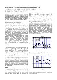
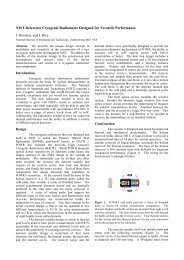
Figure 3: 1-ε(tot) versus D 2 . Diamonds: T(x) =0 K, squares: low,
triangles: high, crosses: isothermal T(x) = T cav
1 - ε(λ) x 10 -6
1400
1200
1000
800
600
400
200
0
0 10 20 30 40 50 60 70
Aperture diameter D 2 / mm 2
1000
900
800
700
600
500
400
300
200
100
0
0 500 1000 1500 2000 2500 3000
Wavelength λ / nm
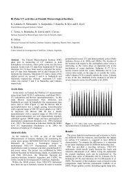
Figure 4: 1-ε(λ) versus λ. Diamonds: 8 mm-low, squares: 8
mm-high, triangles: 3 mm-low, crosses: 3 mm-high
D
mm
∆T cav (h,l,650)
mK
∆T cav (av,0,650)
mK
3 3.5 6.1
8 91 248
λ
nm
∆T cav (h,l,3)
mK
∆T cav (h,l,8)
mK
250 1.5 51
1000 6.3 114
2500 9.3 125
Table 1: Variation ∆T cav in apparent cavity temperature T cav with
T(x) for different cavity diameters D and wavelengths λ. Details
are given in the text.
Finally in the lower half of Table 1 we show ∆T cav (h,l,3)
and ∆T cav (h,l,8) , for D = 3 mm and D = 8 mm, respectively,
associated with the variation of ε(λ) with T(x) between the
high and low profile , shown in Figure 4, for wavelengths
between 250 nm and 2500 nm. All of the results compiled in
Table 1 are based upon the Wien approximation.
Figures 2 to 4 clearly show the influence of the
furnace-temperature profile T(x) on the calculated
emissivities. The upper curve in Figures 2 and 3 is
representative for the ‘cavity only’, T(x) = 0 K; the effect of
the furnace is bending this curve downwards, and the more
the ‘higher’ the profile. Below about D = 3 mm the
differences 1-ε (λ) and 1 - ε(tot) are only slightly
dependent on T(x) but beyond 3 mm we see a marked
variation of the curves with T(x) and -for 1-ε (λ)- to a lesser
extent with wavelength λ. These observations are reflected
by the results shown in Table 1. The variation in apparent
cavity temperature T cav with T(x) for D = 8 mm is
considerably larger than that for D = 3 mm.
This is all in all a strong argument for keeping the cavity
emissivity ε cav as close as possible to unity which -at least
in the present cavity-furnace configuration- would imply
keeping the diameter D of the cavity aperture below about 3
mm. The last column, upper half, of Table 1, showing the
variation ∆T cav (av, 0, 650) for D = 3 mm and D = 8 mm is
noteworthy, since thus far cavity emissivities have been
associated with the profile T(x) = 0 K, cavity only. The
effect of the cavity aperture D -at a given cavity-furnace
configuration- on the temperature distribution within the
cavity will be discussed elsewhere.
It should be stressed that the prime parameter governing the
contribution of the furnace to the overall emissivity is the
cavity emissivity ε cav rather than D 2 . Volume and shape of
the cavity for a given D could be further optimized -within
the restrictions set by the furnace- so as to increase ε cav (D)
and thereby reducing the contribution of the furnace. This
would open opportunities for utilizing fixed-point radiators
with relatively large cavity apertures, when fitted into the
proper furnace.
Conclusions
From the above it can be concluded that heat exchange
between cavity and furnace precludes treating the cavity as
a separate unit. It has to be taken as an integral part of the
furnace-cavity combination making up the radiator.
Acknowledgements
We are indebted to Dr. Alexander Prokhorov for consulting us on
the use of the software package STEEP-3. We wish to thank Dr.
Naohiko Sasajima of NMIJ for the information on the furnace and
its temperature distribution.
References
[1] Prokhorov, A.V., ‘Monte Carlo method in optical
radiometry’, Metrologia, 35, 1998, pp. 465-471.
[2] Yamada Y., Sasajima N., Gomi H., Sugai T., ‘Hightemperature
furnace systems for realizing metal-carbon
eutectic fixed points‘ TMCSI, 7, 2003, pp. 965-990.
284