fusion of absolute vision-based localization and visual odometry for ...
fusion of absolute vision-based localization and visual odometry for ...
fusion of absolute vision-based localization and visual odometry for ...

You also want an ePaper? Increase the reach of your titles
YUMPU automatically turns print PDFs into web optimized ePapers that Google loves.
FUSION OF ABSOLUTE VISION-BASED LOCALIZATION AND VISUAL ODOMETRY<br />
FOR SPACECRAFT PINPOINT LANDING<br />
Bach Van Pham 1 , Simon Lacroix 1 , Michel Devy 1 , Thomas Voirin 2 , Marc Drieux 3 , <strong>and</strong> Clement Bourdarias 3<br />
1 CNRS ; LAAS ; 7 avenue du colonel Roche, F-31077 Toulouse, France<br />
1 Université de Toulouse ; UPS , INSA , INP, ISAE ; LAAS ; F-31077 Toulouse, France<br />
2 European Space Agency, ESTEC - Keplerlaan 1 - P.O. Box 299 - 2200 AG Noordwijk ZH, The Netherl<strong>and</strong>s<br />
3 EADS-ASTRIUM, 66 Route de Verneuil, Les Mureaux Cedex , 78133, France<br />
ABSTRACT<br />
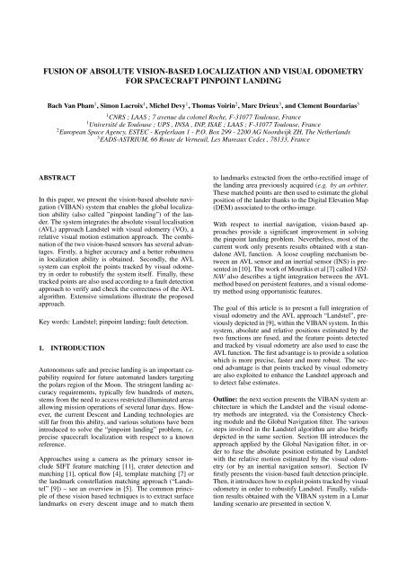
In this paper, we present the <strong>vision</strong>-<strong>based</strong> <strong>absolute</strong> navigation<br />
(VIBAN) system that enables the global <strong>localization</strong><br />
ability (also called ”pinpoint l<strong>and</strong>ing”) <strong>of</strong> the l<strong>and</strong>er.<br />
The system integrates the <strong>absolute</strong> <strong>visual</strong> localisation<br />
(AVL) approach L<strong>and</strong>stel with <strong>visual</strong> <strong>odometry</strong> (VO), a<br />
relative <strong>visual</strong> motion estimation approach. The combination<br />
<strong>of</strong> the two <strong>vision</strong>-<strong>based</strong> sensors has several advantages.<br />
Firstly, a higher accuracy <strong>and</strong> a better robustness<br />
in <strong>localization</strong> ability is obtained. Secondly, the AVL<br />
system can exploit the points tracked by <strong>visual</strong> <strong>odometry</strong><br />
in order to robustify the system itself. Finally, these<br />
tracked points are also used according to a fault detection<br />
approach to verify <strong>and</strong> check the correctness <strong>of</strong> the AVL<br />
algorithm. Extensive simulations illustrate the proposed<br />
approach.<br />
Key words: L<strong>and</strong>stel; pinpoint l<strong>and</strong>ing; fault detection.<br />
1. INTRODUCTION<br />
Autonomous safe <strong>and</strong> precise l<strong>and</strong>ing is an important capability<br />
required <strong>for</strong> future automated l<strong>and</strong>ers targeting<br />
the polars region <strong>of</strong> the Moon. The stringent l<strong>and</strong>ing accuracy<br />
requirements, typically few hundreds <strong>of</strong> meters,<br />
stems from the need to access restricted illuminated areas<br />
allowing mission operations <strong>of</strong> several lunar days. However,<br />
the current Descent <strong>and</strong> L<strong>and</strong>ing technologies are<br />
still far from this ability, <strong>and</strong> various solutions have been<br />
introduced to solve the “pinpoint l<strong>and</strong>ing” problem, i.e.<br />
precise spacecraft <strong>localization</strong> with respect to a known<br />
reference.<br />
Approaches using a camera as the primary sensor include<br />
SIFT feature matching [11], crater detection <strong>and</strong><br />
matching [1], optical flow [4], template matching [7] or<br />
the l<strong>and</strong>mark constellation matching approach (“L<strong>and</strong>stel”<br />
[9]) – see an overview in [5]. The common principle<br />
<strong>of</strong> these <strong>vision</strong> <strong>based</strong> techniques is to extract surface<br />
l<strong>and</strong>marks on every descent image <strong>and</strong> to match them<br />
to l<strong>and</strong>marks extracted from the ortho-rectified image <strong>of</strong><br />
the l<strong>and</strong>ing area previously acquired (e.g. by an orbiter.<br />
These matched points are then used to estimate the global<br />
position <strong>of</strong> the l<strong>and</strong>er thanks to the Digital Elevation Map<br />
(DEM) associated to the ortho-image.<br />
With respect to inertial navigation, <strong>vision</strong>-<strong>based</strong> approaches<br />
provide a significant improvement in solving<br />
the pinpoint l<strong>and</strong>ing problem. Nevertheless, most <strong>of</strong> the<br />
current work only presents results obtained with a st<strong>and</strong>alone<br />
AVL function. A loose coupling mechanism between<br />
an AVL sensor <strong>and</strong> an inertial sensor (INS) is presented<br />
in [10]. The work <strong>of</strong> Mourikis et al [7] called VISI-<br />
NAV also describes a tight integration between the AVL<br />
method <strong>based</strong> on persistent features, <strong>and</strong> a <strong>visual</strong> <strong>odometry</strong><br />
method using opportunistic features.<br />
The goal <strong>of</strong> this article is to present a full integration <strong>of</strong><br />
<strong>visual</strong> <strong>odometry</strong> <strong>and</strong> the AVL approach “L<strong>and</strong>stel”, previously<br />
depicted in [9], within the VIBAN system. In this<br />
system, <strong>absolute</strong> <strong>and</strong> relative positions estimated by the<br />
two functions are fused, <strong>and</strong> the feature points detected<br />
<strong>and</strong> tracked by <strong>visual</strong> <strong>odometry</strong> are also used to ease the<br />
AVL function. The first advantage is to provide a solution<br />
which is more precise, faster <strong>and</strong> more robust. The second<br />
advantage is that points tracked by <strong>visual</strong> <strong>odometry</strong><br />
are also exploited to enhance the L<strong>and</strong>stel approach <strong>and</strong><br />
to detect false estimates.<br />
Outline: the next section presents the VIBAN system architecture<br />
in which the L<strong>and</strong>stel <strong>and</strong> the <strong>visual</strong> <strong>odometry</strong><br />
methods are integrated, via the Consistency Checking<br />
module <strong>and</strong> the Global Navigation filter. The various<br />
steps involved in the L<strong>and</strong>stel algorithm are also briefly<br />
depicted in the same section. Section III introduces the<br />
approach applied by the Global Navigation filter, in order<br />
to fuse the <strong>absolute</strong> position estimated by L<strong>and</strong>stel<br />
with the relative motion estimated by the <strong>visual</strong> <strong>odometry</strong><br />
(or by an inertial navigation sensor). Section IV<br />
firstly presents the <strong>vision</strong>-<strong>based</strong> fault detection principle.<br />
Then, it introduces how to exploit points tracked by <strong>visual</strong><br />
<strong>odometry</strong> in order to robustify L<strong>and</strong>stel. Finally, validation<br />
results obtained with the VIBAN system in a Lunar<br />
l<strong>and</strong>ing scenario are presented in section V.
2. GLOBAL ARCHITECTURE<br />
2.2. L<strong>and</strong>stel<br />
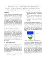
Figure 1. The VIBAN system architecture.<br />
Figure 1 presents the VIBAN system architecture with<br />
two main components: the <strong>visual</strong> <strong>odometry</strong> <strong>and</strong> the L<strong>and</strong>stel<br />
functions. The outputs <strong>of</strong> <strong>visual</strong> <strong>odometry</strong> are firstly<br />
used to enhance the global position estimation provided<br />
by L<strong>and</strong>stel via the Global Navigation filter. Then, these<br />
outputs are also used to make the integrated system more<br />
robust, by directly feeding this in<strong>for</strong>mation into L<strong>and</strong>stel.<br />
Finally, the <strong>visual</strong> <strong>odometry</strong> outputs are used to verify the<br />
output <strong>of</strong> the L<strong>and</strong>stel function in the Consistency Checking<br />
module.<br />
2.1. Visual Odometry<br />
The first <strong>visual</strong> <strong>odometry</strong> ever to be used in a spatial<br />
system is the Descent Image Motion Estimation System<br />
(DIMES) [2]. The sensor was implemented on the Mars<br />
Exploration Rovers (MER) in 2003 <strong>and</strong> tracked four corner<br />
points through three sequential images during the<br />
Mars descent to estimate the spacecraft’s ground-relative<br />
horizontal velocity.<br />
Another <strong>visual</strong> <strong>odometry</strong> (the “NPAL” camera) is described<br />
in [3]. The system is <strong>based</strong> on an EKF filter<br />
in which the positions <strong>of</strong> features are included in the<br />
state vector. The output <strong>of</strong> the system is firstly the relative<br />
spacecraft movement in position <strong>and</strong> altitude <strong>and</strong><br />
secondly, the list <strong>and</strong> the positions <strong>of</strong> tracked l<strong>and</strong>marks<br />
through a series <strong>of</strong> descent images.<br />
Note however that the <strong>visual</strong> <strong>odometry</strong> used in this article<br />
is simulated using Sift points matches [6]. Given two<br />
consecutive images, Sift features <strong>of</strong> each image are extracted<br />
<strong>and</strong> compared with each other, which gives a list<br />
<strong>of</strong> matched points between these two images. The step<br />
is repeated from the first till the last image in the descent<br />
series to <strong>for</strong>m a list <strong>of</strong> tracked l<strong>and</strong>marks.<br />
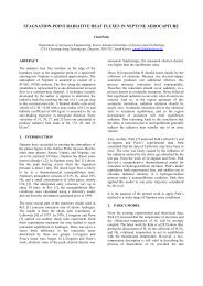
Figure 2. Different steps <strong>of</strong> the L<strong>and</strong>stel algorithm (see<br />
[9] <strong>for</strong> details).<br />
The L<strong>and</strong>stel module is composed <strong>of</strong> one <strong>of</strong>f line <strong>and</strong> one<br />
on line functions. In the <strong>of</strong>f line one, the DEM <strong>and</strong> the associated<br />
2D ortho-image <strong>of</strong> the <strong>for</strong>eseen l<strong>and</strong>ing area are<br />
built from Orbiter images. Initial <strong>visual</strong> l<strong>and</strong>marks are<br />
then extracted in the ortho-image (further denoted as the<br />
”geo image”), using the Difference <strong>of</strong> Gaussian (DoG)<br />
feature points detector [6]. A signature is defined <strong>for</strong> each<br />
extracted feature point. The initial l<strong>and</strong>marks 2D positions,<br />
their signatures <strong>and</strong> their 3D <strong>absolute</strong> co-ordinates<br />
on the planet surface constitute a database stored in the<br />
l<strong>and</strong>er memory be<strong>for</strong>e launch.<br />
The on line function <strong>of</strong> the L<strong>and</strong>stel algorithm consists in<br />
5 steps (figure 2). The first <strong>and</strong> second steps extract <strong>and</strong><br />
trans<strong>for</strong>m the in<strong>for</strong>mation in the descent image so that<br />
the similarity <strong>of</strong> the geometric repartition between the descent<br />
l<strong>and</strong>marks <strong>and</strong> the initial l<strong>and</strong>marks is maximized<br />
(using an homography computed from the altimetry <strong>and</strong><br />
orientation in<strong>for</strong>mation). Then, the third step allows to<br />
extract the signature <strong>of</strong> each descent l<strong>and</strong>mark. The extracted<br />
signature <strong>of</strong> each descent l<strong>and</strong>mark is compared<br />
with the initial l<strong>and</strong>marks signatures (step 4): a list <strong>of</strong><br />
match c<strong>and</strong>idates from the initial l<strong>and</strong>marks set is associated<br />
to each descent l<strong>and</strong>mark. In the last step, a voting<br />
scheme is applied to access the correct matches: several<br />
affine trans<strong>for</strong>mations are extracted within the potential<br />
c<strong>and</strong>idate list, <strong>and</strong> the best affine trans<strong>for</strong>mation (the one<br />
supported by the highest number <strong>of</strong> matches) is used to<br />
generate other matches between descent l<strong>and</strong>marks <strong>and</strong><br />
initial ones.<br />
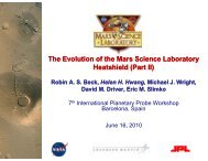
Images on figure 3 show two examples <strong>of</strong> the final<br />
matches obtained by L<strong>and</strong>stel with different illumination<br />
conditions.
where the 0 3 <strong>and</strong> I 3 symbols respectively denote the<br />
3 × 3 null matrix <strong>and</strong> the 3 × 3 identity matrix,<br />
<strong>and</strong> Ω e ie is a skew-symmetric matrix which represents<br />
the planet rotation given by the angular rate<br />
ωie e = [ω 1, ω 2 , ω 3 ] between the planet-centered inertial<br />
frame (i-frame) <strong>and</strong> the planet-centered planetfixed<br />
frame (e-frame):<br />
Ω e ie =<br />
[ ]<br />
0 −ω3 ω 2<br />
ω 3 0 −ω 1<br />
−ω 2 ω 1 0<br />
(3)<br />
Figure 3. Two examples <strong>of</strong> matches provided by L<strong>and</strong>stel<br />
under different illumination conditions. The geo image<br />
(left) is acquired with 55 o − 25 o (azimuth-elevation) sun<br />
position, whereas the descent images (right) are acquired<br />
at 5710m altitude with 145 o −10 o Sun position (a) <strong>and</strong> at<br />
3052m altitude with 235 o −10 o Sun position (b). Zoomed<br />
areas <strong>of</strong> the geo image (center) show the corresponding<br />
matched regions <strong>of</strong> the descent images in the geo one.<br />
<strong>and</strong> Υ = −(Ω e ie Ωe ie − Γe ), Γ e being the short notation<br />
<strong>for</strong> the gravity gradient (the derivative <strong>of</strong> the<br />
gravity). The [a×] represents the misalignment <strong>of</strong><br />
the trans<strong>for</strong>mation matrix between the i-frame <strong>and</strong><br />
the e-frame.<br />
3. Observation: the observation provided by L<strong>and</strong>stel<br />
is the spacecraft position p [9].<br />
⎡<br />
z k = ⎣<br />
[p Global<br />
k<br />
0 2×3<br />
⎤<br />
⎦ (4)<br />
− p L<strong>and</strong>stel<br />
k<br />
]<br />
3. FUSION OF GLOBAL AND RELATIVE POSI-<br />
TION INFORMATION<br />
The main objective <strong>of</strong> the <strong>fusion</strong> between the L<strong>and</strong>stel<br />
<strong>absolute</strong> position estimate <strong>and</strong> the <strong>visual</strong> <strong>odometry</strong> relative<br />
motion estimate, is to yield a more precise <strong>absolute</strong><br />
estimation <strong>of</strong> the spacecraft’s position. This is achieved<br />
thanks to the complementary filter implemented in the<br />
Global Navigation filter (figure 4).<br />
Moreover, the integration <strong>of</strong> the estimated motion provided<br />
by <strong>visual</strong> <strong>odometry</strong>, can allow L<strong>and</strong>stel to focus<br />
the match search within a specific region <strong>of</strong> the geo image<br />
instead <strong>of</strong> searching in the whole l<strong>and</strong>ing area. This<br />
focusing mechanism not only accelerates the algorithm<br />
by reducing the search area, but also improves the algorithm’s<br />
per<strong>for</strong>mance by limiting the false matches probability.<br />
The Kalman filter implemented in the Global Navigation<br />
filter (figure 4) is defined as follows:<br />
<strong>and</strong> the observation matrix is:<br />
H k =<br />
[ 0 0<br />
] 0<br />
0 0 0<br />
1 1 1<br />
Figure 4. The L<strong>and</strong>stel-INS <strong>fusion</strong> principle.<br />
(5)<br />
1. System state:<br />
x = [δΨ T δv T δp T ] (1)<br />
where δΨ is the system attitude’s error, δv the system<br />
speed’s error <strong>and</strong> δp the system position’s error.<br />
Each term is a 3-dimensional vector (3 × 1).<br />
2. Transition matrix:<br />
[ −Ω<br />
e ]<br />
ie 0 3 0 3<br />
Φ k = [a×] −2Ω e ie Υ<br />
0 3 I 3 0 3<br />
(2)<br />
As the Kalman filter used in the Global Navigation filter<br />
is a feed backward filter where the estimated error is<br />
provided to the Global State module after each observation,<br />
the prediction state in this case is always equal to<br />
zero. In reality, the inertial sensors are considered as being<br />
initially calibrated <strong>and</strong> all errors are removed, thus<br />
the prediction state x(1|0) is set to zero. Moreover, after<br />
each estimation with the Kalman filter, the estimated position’s<br />
error is always returned back to the Global State<br />
module <strong>for</strong> correction due to the feed backward mechanism.<br />
As a consequence, the error in the current global<br />
state is considered as being corrected, which results in a<br />
zero prediction state.
The Kalman filter estimates the error in the current estimated<br />
position stored in the Global Navigation filter <strong>and</strong><br />
the uncertainty <strong>of</strong> the estimated global position, provided<br />
by the covariance matrix ˆP k|k−1 .<br />
4. FUSION OF TRACKED POINTS<br />
4.1. Vision-<strong>based</strong> fault detection<br />
Figure 5. This figure illustrates the use <strong>of</strong> the camera<br />
projection function to predict the future positions <strong>of</strong> the<br />
L<strong>and</strong>stel matched points. With L<strong>and</strong>stel, the 3D surface<br />
points D LS are associated to each matched points M in<br />
the descent image. Then, the l<strong>and</strong>er position P 1 at time 1<br />
is estimated as P1 LS . Using the motion estimation δP INS<br />
LS<br />
provided by <strong>visual</strong> <strong>odometry</strong>, the next position ˆP 2 is calculated.<br />
On the basis <strong>of</strong> ˆP 2 <strong>and</strong> D 1 , D 2 , D 3 , the pre-<br />
LS<br />
dicted positions <strong>of</strong> M 1 , M 2 , M 3 at time 2 are calculated<br />
The role <strong>of</strong> the <strong>vision</strong>-<strong>based</strong> fault detection in the Consistency<br />
Checking module is to verify the correctness <strong>of</strong> the<br />
L<strong>and</strong>stel global position estimation. The fault detection<br />
function is <strong>based</strong> on the comparison between the observation<br />
set <strong>and</strong> the prediction set <strong>of</strong> the matched points set<br />
M.<br />
• Prediction Set: using the estimated position returned<br />
by L<strong>and</strong>stel PLS t <strong>and</strong> the motion estimation between<br />
t <strong>and</strong> t + 1 given by <strong>visual</strong> <strong>odometry</strong>, the position<br />
<strong>of</strong> the l<strong>and</strong>er at t + 1 is predicted as ˆP<br />
t+1<br />
LS =<br />
PLS t t+1|t<br />
+ δPINS . As illustrated in figure 5, each point<br />
M k in the set M t , is associated to a 3D point D k on<br />
the surface. The set <strong>of</strong> 3D points matched by L<strong>and</strong>stel<br />
at time t is named D LS . Given the predicted<br />
t+1<br />
position ˆP<br />
LS<br />
<strong>and</strong> the group <strong>of</strong> 3D points D LS, the<br />
positions <strong>of</strong> the M t points in the next image are predicted<br />
using the back projection function. The image<br />
(b) in figure 6 illustrates the predicted positions<br />
<strong>of</strong> the matched points at t in the image acquired at<br />
t + 1 (in red). The prediction set is calculated with:<br />
P re(M t ) = BackP roj(M t t+1<br />
, ˆP<br />
LS , D LS) (6)<br />
= BackP roj(M t , PLS t + δP t+1|t<br />
INS , D LS)<br />
(7)<br />
• Observation Set: given a set <strong>of</strong> the matched points<br />
M t returned by L<strong>and</strong>stel at time t, the set point is<br />
tracked to the next image at time t + 1 with <strong>visual</strong><br />
<strong>odometry</strong>. The left image in figure 6 shows a subset<br />
<strong>of</strong> the matched points returned by the L<strong>and</strong>stel algorithm<br />
(in blue). The right image shows the tracked<br />
points <strong>of</strong> the matched points in the next image (in<br />
green). The observation set is thus obtained via:<br />
Obs(M t ) = T rack(M t , im t , im t+1 ) (8)<br />
Using the observation function in equation 8 <strong>and</strong> the prediction<br />
function in equation 7 (illustrated by the green<br />
<strong>and</strong> red points in figure 6), the L<strong>and</strong>stel output is considered<br />
as being incorrect if the prediction set is inconsistent<br />
with the observation set. Indeed, the observation set depends<br />
only on the nature <strong>of</strong> the two consecutive images<br />
or more precisely on the functionality <strong>of</strong> the <strong>visual</strong> <strong>odometry</strong><br />
which is considered as highly precise <strong>and</strong> reliable at<br />
short term. In contrast, the prediction function does not<br />
exploit the content <strong>of</strong> the two images. In fact, the prediction<br />
set depends only on the output <strong>of</strong> the L<strong>and</strong>stel<br />
algorithm, i.e. the estimated position <strong>and</strong> the associated<br />
3D points. The motion estimation provided by the <strong>visual</strong><br />
<strong>odometry</strong> is also considered as being precise in comparison<br />
with the L<strong>and</strong>stel error during a short period <strong>of</strong> one<br />
second (L<strong>and</strong>stel is operating at 1 Hz).<br />
Let ξ the difference or the innovation between the observation<br />
set <strong>and</strong> the prediction set:<br />
ξ(M t ) = Obs(M t ) − P re(M t ) (9)<br />
The normalized value α <strong>of</strong> the innovation vector ξ(M t )<br />
is calculated with:<br />
α = ξ(M t ) T ∗ P (M t ) −1 ∗ ξ(M t ) (10)<br />
where P (M t ) is the covariance <strong>of</strong> the matched points<br />
M t . The covariance value here indicates the precision<br />
<strong>of</strong> the L<strong>and</strong>stel matched points location, which depends<br />
on the parameters used in the L<strong>and</strong>stel algorithm <strong>and</strong> is<br />
calculated <strong>of</strong>f line. The value α is used to compare with a<br />
predetermined threshold to classify the L<strong>and</strong>stel output.<br />
If the α value is bigger than the threshold, the L<strong>and</strong>stel<br />
output will be reported as erroneous <strong>and</strong> will be discarded,<br />
<strong>and</strong> only the <strong>visual</strong> <strong>odometry</strong> in<strong>for</strong>mation will be<br />
used to propagate the global position estimation – until<br />
L<strong>and</strong>stel retrieves an <strong>absolute</strong> position estimate.<br />
Nevertheless, when the prediction set is consistent with<br />
the observation set, it does not mean that the L<strong>and</strong>stel<br />
output is correct. The L<strong>and</strong>stel output is however then<br />
considered as correct <strong>and</strong> is fed to the Global Navigation<br />
filter, hoping that subsequent steps will retrieve a potential<br />
inconsistency.<br />
4.2. L<strong>and</strong>stel Robustification<br />
The main purpose <strong>of</strong> the L<strong>and</strong>stel Robustification procedure<br />
is to increase the number <strong>of</strong> matched points returned
Figure 6. (a): a descent image with the subset <strong>of</strong> the<br />
L<strong>and</strong>stel matched points. (b): the next descent image<br />
with the L<strong>and</strong>stel interest points tracked by <strong>visual</strong> <strong>odometry</strong><br />
(in green) <strong>and</strong> with the prediction points (in red). For<br />
<strong>visual</strong>ization purpose, only the points matched by L<strong>and</strong>stel<br />
which are successfully tracked by <strong>visual</strong> <strong>odometry</strong> are<br />
shown (23 out <strong>of</strong> 31 here).<br />
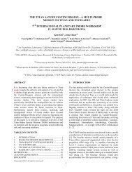
Figure 7. cratered surface with 20 craters/km (named<br />
”NH”) (left) <strong>and</strong> mountainous terrain with 10 km elevation<br />
difference (named ”MB”) (right)<br />
used <strong>for</strong> the two points A <strong>and</strong> B is 160 m/pixel while that<br />
<strong>for</strong> the point C is 80 m/pixel.<br />
by L<strong>and</strong>stel, which consequently improves its precision.<br />
Given a set <strong>of</strong> matched points returned by L<strong>and</strong>stel at one<br />
instant (blue points in figure 6), the set is tracked to next<br />
image with the <strong>visual</strong> <strong>odometry</strong> (green points in figure<br />
6). After having successfully tracked the matched points,<br />
the tracked points are injected into the affine c<strong>and</strong>idates<br />
set <strong>of</strong> the L<strong>and</strong>stel algorithm (output <strong>of</strong> step 5). Then,<br />
the new c<strong>and</strong>idate will be considered as the other normal<br />
c<strong>and</strong>idates. Among these affine c<strong>and</strong>idates, the one with<br />
the highest number <strong>of</strong> matches will be considered as the<br />
best c<strong>and</strong>idate <strong>and</strong> will be used to calculate the position<br />
<strong>of</strong> the spacecraft.<br />
5. RESULTS<br />
5.1. Experiment setup<br />
The purpose <strong>of</strong> these experiments is to analyse the<br />
VIBAN system sensitivity <strong>for</strong> Lunar l<strong>and</strong>ing application<br />
with the PANGU simulator [8]. In these experiments,<br />
the system sensitivity in regard to different parameters as<br />
well as the system per<strong>for</strong>mance analysis are carried on.<br />
Two simulated terrains are used <strong>for</strong> these experiments.<br />
The two simulated terrains used in this experiment. A<br />
cratered surface (named ”NH”) <strong>and</strong> a mountainous terrain<br />
(named ”MB”), are shown in figure 7.<br />
In these experiments, the system is employed during the<br />
Moon transfer orbit coast phase where the l<strong>and</strong>er descends<br />
from 100 kilometres down to 15 kilometres altitude<br />
as shown in figure 8. The l<strong>and</strong>er traverses 5000<br />
kilometres during 1 hour. Due to the long flight time,<br />
the system is only tested at three altitudes which are at<br />
100 kilometres (point A), 58 kilometres (point B) <strong>and</strong><br />
29 kilometres (point C). For each altitude, the system is<br />
employed <strong>for</strong> a time lapse <strong>of</strong> 43 seconds with 1 Hz frequency.<br />
There<strong>for</strong>e, there are 43 images taken <strong>for</strong> each<br />
lapse (also called ”trial”). The orbital image resolution<br />
Figure 8. Lunar Deorbit Phase(image not corresponding<br />
to real scale).<br />
In order to verify the robustness <strong>of</strong> the system with different<br />
levels <strong>of</strong> sensor noise, the experiments are set up with<br />
the following configuration (besides the nominal parameters<br />
described in section 6.6):<br />
1. Camera inclination angle: in this scenario, the embedded<br />
camera angle is about 50 degrees with respect<br />
to the horizon.<br />
2. Image: white noise N (0, 0.005).<br />
3. Radar altimeter: there is no radar altimeter used.<br />
However the l<strong>and</strong>er altitude is known at the beginning<br />
using earth-<strong>based</strong> <strong>localization</strong> with an accuracy<br />
<strong>of</strong> 10 percent. Altitude in<strong>for</strong>mation is then propagated<br />
by pure integration <strong>of</strong> IMU measurement <strong>and</strong><br />
corrected by the VIBAN system.<br />
4. Attitude noise: the INS attitude estimation is considered<br />
as being precise due to the usage <strong>of</strong> the <strong>visual</strong><br />
odometer <strong>and</strong> the star tracker (st<strong>and</strong>ard deviation below<br />
1 ◦ – the L<strong>and</strong>stel has however shown to be able<br />
to cope with 5 ◦ attitude angle errors [9]).
5. Velocity error: the INS velocity error is [1, 1, 1.5]<br />
metres (3σ) in long track, cross track <strong>and</strong> radial axis.<br />
6. Initial position uncertainty: the initial position uncertainty<br />
is set to 5 km <strong>for</strong> both the long track <strong>and</strong><br />
the cross track <strong>for</strong> every point A, B <strong>and</strong> C(worst case<br />
scenario).<br />
5.2. Analysis<br />
5.2.1. Components per<strong>for</strong>mance analysis<br />
In order to show the role <strong>of</strong> each component in the whole<br />
system, the different elements <strong>of</strong> the VIBAN system are<br />
analysed <strong>and</strong> validated one by one. In these tests, the altitude<br />
error is within 10 percent <strong>for</strong> each point A, B <strong>and</strong><br />
C, while the long track <strong>and</strong> cross track error is within a<br />
range <strong>of</strong> 5 kilometres. The sun’s elevation is kept at 1<br />
degree while the difference in azimuth angle between the<br />
descent image <strong>and</strong> orbital map varies from ±45, ±90 degrees<br />
to 180 degrees. In general, there are 5160 images<br />
(120 trials) used <strong>for</strong> these experiments. The cratered surface<br />
NH is used in this test.<br />
By comparing the right chart with the center one, the<br />
number <strong>of</strong> ”false estimation” is reduced from 6 percent<br />
down to 4 percent which means that 38.8 percent <strong>of</strong> faults<br />
are detected. In this case, the number <strong>of</strong> the ”correct estimation”<br />
increases to 70 percent from 68 percent.<br />
As shown by these experiments, a full integration <strong>of</strong> the<br />
L<strong>and</strong>stel sensors with <strong>visual</strong> <strong>odometry</strong> yields a better robustness<br />
<strong>and</strong> accuracy. There<strong>for</strong>e, the full system is used<br />
<strong>for</strong> the following analyses.<br />
5.2.2. Estimation errors<br />
Figures 10 <strong>and</strong> 11 show the position estimation error <strong>of</strong><br />
the VIBAN system <strong>for</strong> the three start points A, B <strong>and</strong> C.<br />
The per<strong>for</strong>mance <strong>of</strong> the system at points A <strong>and</strong> B is equivalent:<br />
this is due to the fact that the orbital image resolution<br />
is the same <strong>for</strong> both case (160 m/pixel). At lower altitude<br />
(point C), the estimation is more precise since the<br />
orbital resolution is doubled. The final estimation error<br />
at the end <strong>of</strong> the trajectory starting at C is approximately<br />
300 metres.<br />
Figure 9. Estimation result with the number <strong>of</strong> ”false”<br />
<strong>and</strong> ”correct” estimations <strong>and</strong> the number <strong>of</strong> images<br />
where the algorithm can not find matches (5160 images<br />
in total). The left chart shows the results obtained with<br />
L<strong>and</strong>stel in a st<strong>and</strong>alone mode, the middle one shows<br />
the result obtained with <strong>visual</strong> <strong>odometry</strong>-L<strong>and</strong>stel position<br />
<strong>fusion</strong>. The right chart shows the results obtained<br />
with the <strong>vision</strong>-<strong>based</strong> fault detection <strong>and</strong> with the L<strong>and</strong>stel<br />
robustification.<br />
Figure 9 illustrates the number <strong>of</strong> image (among 5160<br />
images) where the algorithm can provide a correct estimation,<br />
a false estimation or where the algorithm can not<br />
deliver a position estimation. As shown in the middle<br />
chart <strong>of</strong> the figure, the combination <strong>of</strong> the relative position<br />
estimation computed by the INS (or by a <strong>visual</strong><br />
<strong>odometry</strong>) <strong>and</strong> <strong>of</strong> the global position estimation provided<br />
by L<strong>and</strong>stel shows better per<strong>for</strong>mance than L<strong>and</strong>stel in<br />
a st<strong>and</strong>alone mode. In this case, the number <strong>of</strong> ”false<br />
estimation” is decreased from 26 percent down to 6 percent<br />
thanks to the reduction in the geo image search area.<br />
The number <strong>of</strong> ”no estimation” reduces from 29 percent<br />
down to 26 percent. In fact, the ”no estimation” case is<br />
less dangerous than the ”false estimation” since the l<strong>and</strong>er<br />
can still navigate by integrating IMU measurements.<br />
Figure 10. VIBAN per<strong>for</strong>mance with NH surface at 100,<br />
58 <strong>and</strong> 29 km altitude.<br />
Figure 11. VIBAN per<strong>for</strong>mance with mountainous terrain<br />
MB at 100, 58 <strong>and</strong> 29 km altitude<br />
However, with respect to the mountainous surface MB,
the per<strong>for</strong>mance <strong>of</strong> the system at 100 km altitude is better<br />
than that at 58 km <strong>and</strong> is equal to that at 29 km. The<br />
reason <strong>of</strong> this phenomenon is due to firstly the ratio between<br />
the l<strong>and</strong>er altitude <strong>and</strong> the terrain height variation.<br />
In fact, the L<strong>and</strong>stel algorithm assumes that the surface is<br />
flat, since a homography is applied to the image to be<strong>for</strong>e<br />
establishing the matches. At small altitudes, the mountainous<br />
terrain MB violates this assumption. Secondly,<br />
at high altitude the camera perceives more terrain, which<br />
facilitates the l<strong>and</strong>mark matching process.<br />
5.2.3. Influence <strong>of</strong> the sun position<br />
relatively high. In this test, the mountainous surface MB<br />
is used. The sun condition <strong>for</strong> the ortho image is set at<br />
25 degrees elevation <strong>and</strong> 55 degrees azimuth. The l<strong>and</strong>ing<br />
images are acquired with the sun whose condition is<br />
respectively set at (55,25), (40,10), (40,40), (70,10) <strong>and</strong><br />
(70,40) (azimuth, elevation) degrees. Similarly to the first<br />
scenario, the experiment is also made with images acquired<br />
at 100, 58 <strong>and</strong> 29 km. Figure 13 shows the average<br />
estimation error with the different illumination conditions:<br />
the estimation error is minimized if the l<strong>and</strong>ing<br />
image illumination is identical to that <strong>of</strong> the orbital image.<br />
However, different illumination conditions have little<br />
impact on the system per<strong>for</strong>mance.<br />
In this part, the VIBAN sensitivity to the sun parameters<br />
is analysed. The first experiments study the impact<br />
<strong>of</strong> the illumination difference between the orbital image<br />
<strong>and</strong> the l<strong>and</strong>ing image. The second experiments study the<br />
impact <strong>of</strong> the incidence angle between the camera orientation<br />
<strong>and</strong> the sun’s azimuth.<br />
5.2.4. L<strong>and</strong>er-Orbital Images Illumination<br />
Figure 13. VIBAN average estimation error with 5 different<br />
l<strong>and</strong>ing illumination with mountainous surface MB.<br />
5.2.5. L<strong>and</strong>er/Sun Orientation<br />
Figure 12. VIBAN average estimation error with 5 different<br />
l<strong>and</strong>ing illuminations, with the cratered surface NH.<br />
Two scenarios are evaluated here. The first one analyses<br />
the illumination condition at the Moon poles:, the<br />
cratered surface NH is more appropriate <strong>and</strong> is used in<br />
this test. The sun direction <strong>for</strong> the orbital image is kept<br />
at 5 degrees elevation <strong>and</strong> 0 degree azimuth while the sun<br />
elevation <strong>for</strong> the l<strong>and</strong>ing image is kept at 1 degree <strong>and</strong><br />
the azimuth angles are set a 45, 90, 180, 270 (or -90) <strong>and</strong><br />
315 (or -45) degrees. The test is made with the image<br />
acquired at all <strong>of</strong> the three points A,B,C (100, 58 <strong>and</strong> 29<br />
km altitude). Figure 12 shows the average estimation error<br />
with respect to different l<strong>and</strong>ing sun condition <strong>of</strong> the<br />
VIBAN system. As expected, the bigger the difference<br />
between the ortho <strong>and</strong> l<strong>and</strong>ing images, the bigger the estimation<br />
error is. However, the VIBAN can still operates<br />
in such conditions.<br />
The second scenario represents a typical condition in the<br />
middle <strong>of</strong> the coasting phase where the sun elevation is<br />
Here we analyse the incidence angle between the l<strong>and</strong>er<br />
camera orientation <strong>and</strong> the sun direction. In this analysis,<br />
the cratered surface NH is used. The estimation error is<br />
calculated with the different incidence angle. Figure 14<br />
illustrates the average estimation error with the different<br />
incidence angles, <strong>and</strong> shows that the VIBAN system perturbed<br />
when the sun is directly in front <strong>of</strong> the spacecraft.<br />
In this situation, the embedded camera can only perceive<br />
the craters rim. There<strong>for</strong>e, the l<strong>and</strong>ing image content is<br />
poorer than with other incidence angles. Figure 14 also<br />
shows that there is no difference in the system per<strong>for</strong>mance<br />
with incidence angle smaller than 90 degrees. The<br />
final estimation error <strong>for</strong> the worst case is about 1500 metres<br />
(at 100 kilometres altitude) while the best final estimation<br />
error is about 1000 metres.<br />
5.2.6. Nominal Scenarios<br />
Contrary to the previous analyses where there is no connection<br />
between the three points A, B <strong>and</strong> C, the nominal<br />
scenario tries to analyse the VIBAN system within<br />
a whole coasting trajectory. The estimation error at the<br />
one <strong>of</strong> the two points B (respectively C) inherits from the
Figure 14. VIBAN estimation error with cratered surface<br />
NH at 100 kilometres altitude, using different sun/l<strong>and</strong>er<br />
incidence angle.<br />
VIBAN estimation applied <strong>for</strong> the trajectory starting at<br />
point A (respectively B).<br />
Figure 16. Nominal<br />
gation period using the INS or <strong>visual</strong> <strong>odometry</strong> between<br />
the two points A <strong>and</strong> B or B <strong>and</strong> C isn’t shown due to the<br />
large difference in time scale (129 seconds versus 2500<br />
seconds). The relative navigation error results in high<br />
jumps in the estimation error at the 43 rd second <strong>and</strong> at<br />
the 86 th second. As explained above, the second scenario<br />
yields larger estimation errors at the beginning <strong>of</strong><br />
the coasting phase due to the front sun situation. However,<br />
the difference in the estimation error at the end <strong>of</strong><br />
point A is corrected at the beginning <strong>of</strong> point B. The final<br />
average estimation errors in magnitude <strong>for</strong> the two scenarios<br />
1 <strong>and</strong> 2 are respectively 245 metres <strong>and</strong> 293 metres<br />
([151 149 38] <strong>and</strong> [186 164 28] in long track, cross<br />
track <strong>and</strong> altitude). Trials with lower altitudes showed<br />
that VIBAN can yield smaller estimation errors.<br />
6. CONCLUSIONS<br />
Figure 15. The two nominal scenarios<br />
Two scenarios are defined <strong>for</strong> this analysis (figure 15). In<br />
the first scenario, the l<strong>and</strong>er follows the transition <strong>of</strong> the<br />
Moon dark <strong>and</strong> bright sides from the North Pole down<br />
to the South Pole. The sun/l<strong>and</strong>er incidence angle is set<br />
to 45 degrees <strong>for</strong> the points A <strong>and</strong> C (corresponding to<br />
North <strong>and</strong> South Pole). For the second scenario, as illustrated<br />
in figure 15, the l<strong>and</strong>er faces the sun at point A (i.e.<br />
180 degrees sun incidence angle). At point C, the sun is<br />
directly behind the l<strong>and</strong>er. The difference in illumination<br />
between the l<strong>and</strong>ing image <strong>and</strong> the orbital image varies<br />
from 45 degrees to 345 degrees. The initial position error<br />
at point A is set to (1.6; 1.6;0.1) km <strong>for</strong> long track, cross<br />
track <strong>and</strong> altitude.<br />
Figure 16 shows the average estimation error <strong>of</strong> five runs<br />
with the two scenarios. Since at each point A, B <strong>and</strong> C,<br />
the L<strong>and</strong>stel sensor is used with a time lapse <strong>of</strong> 43 seconds,<br />
there are in total 129 estimation results. The navi-<br />
In this paper, we have demonstrated the benefits <strong>of</strong> the<br />
coupling mechanism between an <strong>absolute</strong> <strong>vision</strong>-<strong>based</strong><br />
<strong>localization</strong> algorithm (L<strong>and</strong>stel) <strong>and</strong> a <strong>visual</strong> <strong>odometry</strong><br />
method. Similarly to an INS-GPS <strong>fusion</strong> problem, the<br />
<strong>fusion</strong> between the global estimation computed by the<br />
L<strong>and</strong>stel module <strong>and</strong> the local estimation provided by <strong>visual</strong><br />
<strong>odometry</strong>, not only improves the <strong>localization</strong> precision<br />
but also enhances the system’s overall per<strong>for</strong>mance<br />
in term <strong>of</strong> speed <strong>and</strong> robustness. Besides these advantages,<br />
the use <strong>of</strong> the points tracked by <strong>visual</strong> <strong>odometry</strong><br />
also robustifies the L<strong>and</strong>stel per<strong>for</strong>mances.<br />
Moreover, using <strong>visual</strong> <strong>odometry</strong> in the system instead<br />
<strong>of</strong> conventional INS permits the introduction <strong>of</strong> a <strong>vision</strong><strong>based</strong><br />
fault detection approach, which can prevent the<br />
system from using the incorrect in<strong>for</strong>mation provided<br />
by the <strong>absolute</strong> <strong>visual</strong> <strong>localization</strong> method. In fact, this<br />
<strong>vision</strong>-<strong>based</strong> fault detection system can not only be used<br />
with the L<strong>and</strong>stel function but can also be coupled with<br />
other <strong>vision</strong>-<strong>based</strong> global position estimation solutions,<br />
like the crater detection, the template matching or the optical<br />
correlation approaches.
REFERENCES<br />
[1] Yang Cheng <strong>and</strong> Adnan Ansar. L<strong>and</strong>mark <strong>based</strong><br />
position estimation <strong>for</strong> pinpoint l<strong>and</strong>ing on mars.<br />
Proceedings <strong>of</strong> the 2005 IEEE International Conference<br />
on Robotics <strong>and</strong> Automation, pages 1573 –<br />
1578, 2005.<br />
[2] Yang Cheng, Andrew Johnson, <strong>and</strong> Larry Matthies.<br />
Mer-dimes: a planetary l<strong>and</strong>ing application <strong>of</strong> computer<br />
<strong>vision</strong>. Computer Vision <strong>and</strong> Pattern Recognition,<br />
2005.<br />
[3] B. Frapard, B. Polle, G. Fl<strong>and</strong>in, P. Bernard,<br />
C. Vetel, X. Sembely, <strong>and</strong> S. Mancuso. Navigation<br />
<strong>for</strong> planetary approach <strong>and</strong> l<strong>and</strong>ing. 5th Int.<br />
ESA Conf. Spacecraft Guidance., Navigation. Control<br />
System, 2002.<br />
[4] K. Janscheck, V. Techernykh, <strong>and</strong> M. Beck. Per<strong>for</strong>mance<br />
analysis <strong>for</strong> <strong>visual</strong> planetary l<strong>and</strong>ing navigation<br />
using optical flow <strong>and</strong> dem matching. AIAA<br />
Guidance, Navigation <strong>and</strong> Control, 2006.<br />
[5] Andrew E. Johnson <strong>and</strong> James F. Montgomery.<br />
Overview <strong>of</strong> terrain relative navigation approaches<br />
<strong>for</strong> precise lunar l<strong>and</strong>ing. IEEE Aerospace Conference,<br />
2008.<br />
[6] David Lowe. Object recognition from local scaleinvariant<br />
features. ICCV, 1999.<br />
[7] Anastasios I. Mourikis, Nikolas Trawny, Stergios I.<br />
Roumeliotis, Andrew E. Johnson, Adnan Ansar,<br />
<strong>and</strong> Larry Matthies. Vision-aided inertial navigation<br />
<strong>for</strong> spacecraft entry, descent, <strong>and</strong> l<strong>and</strong>ing. Trans.<br />
Rob., 25(2):264–280, 2009.<br />
[8] S.M Parkes, I. Martin, M. Dunstan, <strong>and</strong><br />
D. Matthews. Planet surface simulation with<br />
pangu. SpaceOps, 2004.<br />
[9] Bach Van Pham, Simon Lacroix, Michel Devy,<br />
Marc Drieux, <strong>and</strong> Christian Philippe. Visual l<strong>and</strong>mark<br />
constellation matching <strong>for</strong> spacecraft pinpoint<br />
l<strong>and</strong>ing. AIAA Guidance, Navigation <strong>and</strong> Control,<br />
2009.<br />
[10] Bach Van Pham, Simon Lacroix, Michel Devy,<br />
Marc Drieux, <strong>and</strong> Thomas Voirin. L<strong>and</strong>mark constellation<br />
matching <strong>for</strong> planetary l<strong>and</strong>er <strong>absolute</strong> <strong>localization</strong>.<br />
International Conference on Computer<br />
Vision Theory <strong>and</strong> Application, 2010.<br />
[11] Nikolas Trawny, Anastasios I. Mourikis, Stergios I.<br />
Roumeliotis, Andrew E. Johnson, <strong>and</strong> James Montgomery.<br />
Vision-aided inertial navigation <strong>for</strong> pinpoint<br />
l<strong>and</strong>ing using observations <strong>for</strong> mapped l<strong>and</strong>marks.<br />
Journal <strong>of</strong> Fields Robotics, 2006.