x–ray computed tomography inspection of the stardust heat shield

X–RAY COMPUTED TOMOGRAPHY INSPECTION OF THE STARDUST
HEAT SHIELD
(IPPW-7)
Karen M. McNamara (1) , Daniel J. Schneberk (2) , Daniel M. Empey (3) *, Ajay Koshti (1) , D. Elizabeth Pugel (4) , Ioana
Cozmuta (5) , Mairead Stackpoole (5) , Norman P. Ruffino (6) , Eddie C. Pompa (6) , Ovidio Oliveras (6) and Dean A.
Kontinos (7)
(1) NASA Johnson Space Center, (2) Lawrence Livermore National Labs, (3) Sierra Lobo, Inc., (4) NASA Goddard Space
Flight Center, (5) Eloret Corporation, (6) Jacobs Technology, (7) NASA Ames Research Center
ABSTRACT
The “Stardust” heat shield, composed of a PICA
(Phenolic Impregnated Carbon Ablator) Thermal
Protection System (TPS), bonded to a composite
aeroshell, contains important features which chronicle
its time in space as well as re-entry. To guide the
further study of the Stardust heat shield NASA
reviewed a number of techniques for inspection of the
article. The goals of the inspection were: 1) to
establish the material characteristics of the shield and
shield components, 2) record the dimensions of shield
components and assembly as compared with the preflight
condition, and 3) through the evaluation of the
shield material provide input to future missions which
employ similar materials.
1. INTRODUCTION
The recently returned “Stardust” heat shield contains
important features which chronicle its time in space as
well as re-entry. To guide the further study of the
Stardust shield NASA reviewed a number of nondestructive
techniques for inspection of the shield. The
goals of the inspection are: 1) to establish the material
characteristics of the shield and shield components, 2)
record the dimensions of shield components and
assembly as compared with the pre-flight condition,
and 3) through the evaluation of the shield material
provide input to future missions which employ similar
materials.
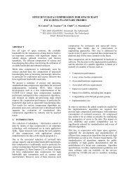
Industrial X-Ray Computed Tomography (CT) is a 3D
inspection technology which can provide information
on material integrity, material properties (density) and
dimensional measurements of the heat shield
components. Computed tomographic volumetric
inspections can generate a dimensionally correct,
quantitatively accurate volume of the shield assembly.
Because of the capabilities offered by X-ray CT,
NASA chose to use this method to evaluate the
Stardust heat shield.
Personnel at NASA Johnson Space Center (JSC) and
Lawrence Livermore National Labs (LLNL) recently
performed a full scan of the Stardust heat shield using a
newly installed X-ray CT system at JSC. This paper
briefly discusses the technology used and then presents
the results of the scans obtained along with
comparisons of the scan data with data obtained from
samples cut from the heat shield as well as
comparisons with the as-built dimensions. Density
variation, “char” layer thickness, recession and bond
line (the adhesive layer between the PICA and the
aeroshell) integrity are all evaluated. Finally
suggestions are made as to future uses of this
technology as a tool for non-destructively inspecting
and verifying both pre and post flight heat shields.
Fig. 1 - Stardust Capsule.
Industrial X-Ray Computed Tomography is a 3D
inspection technology which can provide information
on material integrity and dimensional measurements of
shield components and component materials.
Computed tomographic volumetric inspections can
generate a dimensionally correct, quantitatively
accurate volume of the shield assembly. CT
reconstructed data is comprised of volume elements or
“voxels” at each 3D position in the volume covering
the object under inspection. For x-ray based CT the
voxel is in units of x-ray attenuation, relative
attenuation for polychromatic sources and total
attenuation for mono-chromatic sources; the product of

chemical formula and density. Consequently, voxel
intensities measure changes in material composition
and can be used to measure dimensions of features,
anomalies and/or component structures.
NASA JSC has recently completed the construction of
an x-ray cell facility that includes two x-ray sources
and two detectors. The two x-ray sources are a
COMET 450 KVp tube with focal spots of 0.4 and 1.0
mm, and a 150 KVp Hamamatsu Micro-Focal source
with three choices of x-ray spot (0.05, 0.01 and 0.005
mm nominal). The COMET tube head is on a
manually translatable rail which supports source-todetector
distances from 4 to 12 feet. The Hamamatsu
micro-focal source resides on the 4 ft by 6 ft optical
table with the THALES Amorphous Silicon detector,
enabling precise positioning for high-cone angle
techniques. Up to three different NEWPORT motion
stages are also on the optical table to support different
Computed Tomography and Laminographic scanning
methodologies. Taken as a whole, the two x-ray
sources, the manual and computerized motion; the JSC
X-ray capability can scan a large variety of objects, at a
wide range of spatial resolutions, and employing a
range of scanning techniques.
2. SCANNING METHODOLOGY
The diameter of the Stardust shield is 81 cm (32 in.)
with the overall shape of a blunted 60° half angle
sphere cone.. Further, the Stardust shield can be
described as constituted of 3 layers; 1) an outer PICA
layer, 2) an Aluminum honeycomb layer and 3) a
support substructure of aluminum posts and interior
cross-members. Inspection questions span the different
components of the shield; what is the material state of
the PICA, what is the material thickness, and is this
thickness greater or less in different parts of the shield?
Is there a change in the material composition of the
PICA close to the exterior surface? What is the
magnitude of this change? Are there any unexpected
anomalies in the Aluminum honeycomb? And, what is
the state of the bond-line between the PICA and the
Aluminum honeycomb.
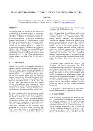
The 450 kVp scanning system at JSC includes motion
can accommodate 4 different scanning modes. Figure
2 contains the different alternatives. Given the large
size of the Stardust shield as compared to the 40 by 30
cm (approximately 16 by 12 in.) size of the Flashscan
33 detector, we elected to implement a ‘tiled-scan”
strategy. The impact of this choice is rather long scan
times; the total scan time equals the time for a single
scan multiplied by the number of tiles. Secondly, there
is the added complexity of positioning the detector
with sufficient precision to construct a “joined” scan
that does not include artifacts from the “joining”
operation. The source-detector geometry for the JSC
450 kVp room is cone-beam, requiring the detector be
moved to cover the entire projected size of the Stardust
shield at the detector plane. To reduce the number of
tiles we elected to scan with “half-scan” or “offsetscan”
techniques where we reconstruct the entire object
from a field of view that covers just over half of the
X-ray
Source
X-ray
Detector
X-ray
Source
X-ray
Detector
ROI Scan – part centered – scanner aligned
Half-Scan – part centered – scanner aligned
X-ray
Source
X-ray
Detector
X-ray
Source
X-ray
Detector
in 4 Tiles
Overlap
Overlap
ROI Scan – single-end – scanner aligned –
180 plus two fan-angles Tiled-CT – part centered – scanner aligned
Fig. 2 - Alternative scanning modes at JSC.
Overlap

object. These two techniques result in a scan
comprised of three separate “scan-tiles”, which when
joined together and reconstructed produce a 3D CT
volumetric inspection data set for the Stardust shield.
Selected scan parameters for each of the tiled scans
represent a choice among competing constraints. The
virtual detector is built up from the different scans,
resulting in large data sets. Consequently, the number
of rotational views acquired should be sufficient for the
constructed detector, not any one tile. It is important to
note also that increasing the number of views increases
scan time by the number of tiles. Secondly, alignment
tolerances get more critical with cone-angle which
increases the amount of precision for positioning the
detector. Third, we are interested in substantial spatial
resolution, which means the source unsharpness (the
blur due to the finite size of the source spot) needs to
be kept under control. These constraints given, we
elected to scan the shield with 900 views over 360
degrees. We are looking for spatial resolution in the
0.3-0.5 mm range, consequently we chose to position
the source-object-detector in a low-cone, lowmagnification
configuration. The source to detector
distance was set at 3048 mm, with a source to object
distance of 2591 mm, an x-ray magnification of 1.176.
The amorphous silicon detector was operated in the 1.5
binning mode, resulting in a detector size of 0.1905
mm at the detector, and with this magnification, the
voxel size for the reconstructed volume could be as
low as 0.162 mm. For the virtual detector, comprised
of the 3 tiles, the field of view was roughly 570 mm,
resulting in a cone angle of this configuration resulted
in a cone-angle of 9.4 degrees. Using the small spot
from the COMET tube head of 0.4 mm, the estimated
size of the source unsharpness at the object for this
magnification is 0.0704 mm, easily less than the 0.162
mm minimum voxel size for the reconstructed volume.
Each of the three 900 view scans was acquired
separately with the detector moved in-between scans.
Referring to Fig. 2, the center section scan comprised a
ROI scan, and was acquired first to enable a centerreconstruction
to be processing while the other scantiles
were being acquired. Fig. 3 contains individual
radiographs with the joined radiograph displayed in
Figure 4. Fig. 5 contains a vertical slice from the
reconstructed volume for the Stardust heat shield
inspection.
All 900 radiographs in the three tiles were joined into a
radiograph as displayed in Fig. 4. Those 900
radiographs acquired over 360 degrees were then
processed and reconstructed with a modified Feldkamp
reconstruction algorithm for the “offset-scan”
geometry illustrated by the radiograph in Fig. 5. In the
course of processing the data we resampled the
projection data to support a reconstruction into 0.324
mm cubic voxels (the 0.162 mm pixel radiographs
were resampled 2x2). The result is a 2640 by 2640 by
1000 volume of voxel elements.
Fig. 3 - First images from the three acquired scans.

Fig. 4 - Joined digital radiograph from three tiled scans.
Fig. 5 - Vertical slice from tiled offset-scan.
The vertical slice shown in Fig. 5 shows two of the
main components of the stardust shield, the PICA and
the aluminum honeycomb underneath. Also, notice
some structured noise or artifacts in the lower part of
the vertical slice in Fig. 5 which are a combination of
“streak” artifacts (from the long chords in the
Aluminum and the inadequate number of views for a
radiographic area of this size). Fig. 6 contains a closeup
view of the center-top of the vertical slice from the
reconstructed volume showing the type of detail
imaged by the CT scanning in the JSC system. Using
the different Aluminum pieces, and the drilled holes in
the Stardust Shield as reference standards, the volume
appears to include accurate dimensions of the internals
of the Stardust shield.
3. REVIEW AND ANALYSIS OF 3D
VOLUMETRIC DATA
The 3D CT data can be viewed and unpacked in a
number of different ways from a number of different
orientations. Fig. 7 contains a cross-sectional or
(transverse) slice through the Stardust reconstructed
volume. In both Fig. 6 and Fig. 7, notice the texture in
the slices through the PICA, we consider this texture in
the images to be an accurate measure of the variation
of the fibers in the make-up of the PICA. Also, there
appears to be higher attenuating material sparsely
interspersed within PICA material. Preliminary
analysis of these higher-attenuating chunks indicate a
close resemblance to the same features found in scans
of recently fabricated PICA [1]. Second, notice the

small change in attenuation in the cross-sectional slices
towards the outside boundary of the PICA, we consider
this change in attenuation to be the char layer, a feature
we will examine subsequently. Third, for the slices
showing the state of the Aluminum honeycomb, notice
a variation in the attenuation in the interstitial layer
between the honeycomb and the PICA. It appears
there are gaps in the fill between the PICA and the
Aluminum honeycomb. Fourth, there appears to be
higher attenuating material on the outside of the PICA.
From a visual inspection of the outside of the shield,
this is “dirt” accumulated on the shield from the
landing. As expected the “dirt” is higher in x-ray
attenuation than the PICA. Lastly, notice the hole cut
Fig. 6 - Extracted region from verticle CT slice.
in the PICA from some destructive analysis work. This
feature provided a useful reference for verifying the
dimensional accuracy of our reconstructed volume.
Four questions have been identified as important for
the analysis of the Stardust Shield; 1) what is the
thickness of the PICA layer, and how does it compare
to the as-built state of the shield, 2) are there anomalies
Fig. 7 - Transverse CT slice.
in the PICA layer and can this data be used to estimate
the depth of the char layer in the PICA, 3) what is the
state of the bond-line between the aluminum
honeycomb and the PICA layer, and 4) are there any
features in this data that result from the scanning and
processing techniques, themselves, and how could
these techniques be improved upon for scanning
another shield.
4. MEASUREMENT OF PICA THICKNESS
While there a many ways to measure the thickness of
the PICA layer in the scanned volume, the methods
developed here focus on “point-wise” techniques. That
is, we sought to obtain measurements of the thickness
of the PICA from points on the surface of the PICA.
Unlike “shell-extraction” techniques, or “boundaryfitting”
techniques, these methods do not fit to the
elliptical shape, but rather attempt to measure
boundaries as they are in the data, and calculate the
difference between the boundaries. Our procedure
starts with a “center vertical slice” and then rotates the
volume to obtain measurements from “center vertical
slices” at a large number of angles throughout the
volume. In this way thickness measurements are
obtained over the entire surface of the Stardust Shield.
The measurement procedure for a center vertical slice
involves three steps; 1) measure the coordinates of the
boundary of the outer PICA layer from the center
vertical slice, 2) for the same vertical slice, measure the
boundary of the inner PICA layer (the inner boundary
is bounded by the aluminum honeycomb layer), and 3)
measure the distance from outer to inner boundary on
the line perpendicular to the surface of the outer
boundary. Fig. 8 shows plots of the outer and inner
boundary contours of the PICA layer from the scan of
the Stardust shield obtained from “shrink-wrap”
operations applied to the volume. Fig. 9 shows the
PICA thickness measured from the boundaries in Fig. 8
compared with the “as-built” thickness. Fig. 10 shows
the estimated material loss based on Figs. 8 and 9.
A few trends in the material loss in the PICA are
apparent from the data. First the loss of material
(compared to the assumed build with a constant
thickness) is greater at the top of shield than towards
the outer ends. The maximum loss is around 6.3 mm
(¼ inch) in thickness. But as can be seen from the
outside of the shield there is substantial variation in the
outer texture with “chunks” of the shield missing,
possible due to the impact at landing. However,
independent of the chunks missing from the shield,
there appears to be a near-linear decrease in the loss of
the PICA material proceeding from the top of the
Shield to the outside edges.

Fig. 8 – Plot of inner and outer boundaries of PICA.
Fig. 9 – PICA thickness measurements.

Fig. 10 - PICA thickness loss from nominal thickness of 58 mm.
Applying this technique to the entire volume involves
rotating the scanned volume of the Stardust shield, and
obtaining a sequence of center slices at different
rotational angles. Independent of the debris sticking to
the outside of the shield, and small variations in the
surface of the shield, the trends in the thickness are
reasonably consistent with the indications reported
from a single slice. The center of the shield lost more
material than the outer radii of the shield. These
measurements show a material thickness loss of 6-6.5
mm in the top of the shield apex, and a low as 3 mm
loss close to the outside radii of the shield surface. The
variation in the material loss from top of the dome to
the outer ends is only slightly non-linear, with the loss
in material greatest at the dome, with a more rapid
decrease from top of the dome to the ends, then less
loss at the ends. It should be mentioned here that the
drilled holes in the shield complicate these point-wise
measurements from the CT data, where we are
calculating “tangents” to contours and inverse slopes to
the tangents, which in itself can be unstable (small
values of the tangent results in large numbers in the
inverse).
5. MEASUREMENTS OF THE CHAR LAYER
The “char” layer is a lower attenuating band of PICA
material at the outer boundary of the shield. Fig. 11
includes an image extracted from the top of the dome,
with the grey-level-window set to just span the
attenuation of the PICA (the “dirt” on the outside layer
are all at the maximum gray level). Notice the subtle
differences in density characteristic of this layer. To
obtain a quantitative measure of the density differences
in the charred PICA line-outs were acquired at
different positions indicated on the image. Fig. 12 is a
comparison of the relative attenuation along the line
outs. Since the char layer occupies the region close to
the outside boundary, we obtained “shell-extractions”
from the reconstructed volume. This process involves
finding the outer boundary, then shrinking the outer
boundary to intersect a layer at a uniform distance from
the edge, thereby generating an image of the internals
of the Stardust shield in exclusively in the char layer.
Fig. 13 is an image of the shell extraction of the entire
char layer, Fig. 14 is a extract of the char layer shell,
and Fig. 15 is an extract of a layer deeper into the
PICA.
The variation in the attenuation values in the above
images and displayed in the, images, line-outs, and
histograms shows the difficulty in accurately
dimensioning the char layer. First, there is variation in
the fibers themselves that is close to the change in
density in the char layer (0.000109 for a mean value of
0.00214 – approx 1 part in 20). Second, comparing
average values from a shell extraction in the char layer
and from a layer inside the char (the “no-char” region),
the “char layer is lower in attenuation by about 12%.
However, referring to Fig. 17, notice the substantial
overlap between the histograms of voxels from the char
and no-char layer. This can also be observed in the
images; some of the fibers in the char layer retain their
original density.

Fig. 11 - Extracted section of top dome showing approximate positions of line-outs.
0.0025
0.0024
(mm‐1)
Relative Attenuation
0.0023
0.0022
0.0021
0.002
0.0019
0.0018
0.0017
0.0016
0.0015
0 2 4 6 8 10 12 14 16
Distance (mm)
LineOut‐1
LineOut‐2
LineOut‐3
LineOut‐4
LineOut‐5
Fig. 12 - A comparison of the relative attenuation from the line-outs indicated in Fig. 11.
Fig. 13 - Shell extraction for the entire volume in the outer char layer.

Fig. 14 – Extracted region from the shell of the outer char layer.
Fig. 15 - Extracted region from the shell of the inner layers of PICA well inside the char layer.
160
140
120
N of Occurences
100
80
60
40
20
0
0.0007 0.0012 0.0017 0.0022 0.0027 0.0032
Relative Attenuation
No‐Char
Char‐Layer
Fig. 16 - Histograms from extracted regions of the same size from the shell extraction data.

Third, and as expected, the loss in density in the char
layer results in a material that is less uniform than the
“no-char” region as shown in the width of the
histogram for the “Char-Layer” voxels.
Using the shell extractions we can average along radial
lines, effectively taking line-outs to obtain some
measure of the depth of the char layer. Average depth
of the char layer is 9.8 mm +/- 1mm. Also on average
the char layer is greater at the positions of largest mass
loss, that is, at the “dome” region of the Stardust
Shield. Given all the difficulties mentioned above for
distinguishing the char layer from the “no-char” layer,
and the variation in the density of the PICA, this is
admittedly a measurement with substantial local
variation.
Comparisons of the above numbers with those from the
cores taken from the heat shield are of interest.
Reference [2] estimated the combined char layer and
pyrolysis depth to be ~ 11 mm for the flank core and
~9 mm for the stagnation core, similar to the numbers
above.
Fig. 17 - Cross-sectional slice showing PICA, bondlayer
and Honeycomb.
6. STRUCTURE AND ANOMALIES IN THE
BOND LAYER
The “bond-layer” referred to here is the layer of
material in-between the PICA and the Aluminum
honeycomb. From the cross-sectional slices presented
above and below the layer is higher in attenuation than
the PICA, and is close in attenuation to the Aluminum.
Figure Figs. 17 and 18 contain extracted regions from
cross-sectional slices through the PICA, the section at
the top of the honeycomb and containing the bondlayer.
Notice the small porosity at about 4 o’clock in
the bond-layer in Fig. 17. Also, notice the excess
metal in the honeycomb.
The cross-sectional slice in Figure 18 shows a gap in
the bond-layer at a radial position of 3 o’clock. This
void-space in the “bond-layer” extends a length of
approximately 20 mm at this particular position.
Fig. 18 - Cross-sectional slice showing a gap in the
bond-layer.
.
Fig. 19 - Shell extraction of the bond-layer.

Fig. 20 - Close-up of the top of the image in Fig. 19.
“Shell extractions” utilized above to examine the char
layer can be used to evaluate the bond-layer in the
Stardust heat shield. Using the exterior of the
aluminum honeycomb as a boundary we can position a
shell with this contour in the geometric position of the
“bond-layer”. Consequently, we obtain an image of
the entire “bond-layer’ in one image. Figs. 19 and 20
show this.
The “shell-extraction” images show a number of gaps
in the “bond-layer” in the Stardust heat shield. In
general the bond-line is better filled at the top of the
shield than down the length towards the ends of the
shield. In particular for the section at the top shown in
Fig. 20 the bond-layer is only 62% filled, that is 38%
of the space in the bond layer contains substantial
voids. At this point in time these results have not been
compared to the as-built data so it is not clear if the
void-fraction developed over time in service, or the
void-fraction is as-built
7. ARTIFACTS IN THE CT DATA AND
LESSONS LEARNED
From the evaluation of the entire 3D CT volume two
different types of artifacts can be identified which
hamper the evaluation of certain features in the data.
First, the sections of PICA and aluminum honeycomb
in close proximity to the Aluminum support structure
are inundated with troublesome “streak” artifacts. Fig.
21 contains a cross-sectional slice displaying these
effects in the reconstructed volume. These artifacts are
the result of a “lack of penetration” of the longer
sections of Aluminum in the support structure
combined with the proportion of “Background Scatter”
[3] characteristic of this technique. In many cases
these effects can be remediated by a thicker x-ray beam
filter, thereby increasing the average energy used in the
scanning. This should be considered in subsequent
scanning.
increment must be comparable with the spatial
resolution of the radiographic projection to get all the
Fig. 21 - Cross-sectional slice showing streak artifacts.
resolution available in the radiograph into the 3D
reconstruction. The mathematics result in the
requirement that the number of rotational views be pi
or pi/2 times the number of spatial resolution elements
out to the radius of interest. Given that the PICA is at a
radius of some 900 pixels, it is clear that 900 views are
not adequate to avoid the periodic noise resulting from
the lack of rotational views. The result is an additional
source of noise that makes detailed examination of the
PICA in the wider sections of the shield more difficult.
In subsequent scans the number of views should be
increased to 1200 or 1800 views over 360, provided
part-availability and funding exist for this added scan
time.
Another type of artifact occurs in the sections of the
Stardust Shield down from the top of dome and is due
to the lack of views acquired. There is a relationship
between the radius at which features appear and the
angular increment used to obtain the number of views
for the reconstruction [4]. In particular, the angular

8. SUMMARY
To evaluate the structure of the Stardust Shield a tiled-
CT scan was performed on the Stardust Shield in the
newly fabricated 450 kVp x-ray room at JSC. The
results are varied. First, the results show the loss in the
shield thickness as compared to the as-built thickness
to be 6-6.5 mm in the top of the shield apex, and a low
as 3 mm loss close to the outside radii of the shield
surface. The variation in the material loss from top of
the dome to the outer ends is only slightly non-linear,
with the loss in material greatest at the dome, with a
more rapid decrease from top of the dome to the ends,
then less loss at the ends. Second, CT data showed
indications of a char layer in the PICA on the outside
of the Stardust Shield. The density of the char layer is
less than the unaffected PICA by 12%. Also, the
thickness of the char layer is on average 9.8 mm +/- 1
mm. This measurement includes substantial local
variations with some of the fibers in the char layer near
the attenuation values of the unaffected PICA. The
nature of this variation is difficult to establish without
better data on the as-built material. Lastly, a few
troublesome scan artifacts were identified as part of
these scans. We recommend a thicker x-ray beam filter
and the acquisition of more rotational views. For tiled-
CT scanning increasing the number of rotational views
increases the scan time by the number of tiles, and
could result in substantial increased cost. However, if
the interest of the scan is focused on the top of the
dome where the angular increment and radius
requirements are not as stringent, this scan strategy is
adequate to support the variety of measurements
presented here.
9. REFERENCES
1. Empey D. M. and Schneberk, D. J., Results from
medium resolution and high resolutions scans of PICA,
Working Paper, 2007
2. Stackpoole M., Sepka S., Cozmuta I., Kontinos D.,
Post-Flight Evaluation of Stardust Sample Return
Capsule Forebody Heatshield Material, AIAA-2008-
1202, 46 th AIAA Aerospace Sciences Meeting and
Exhibit, Reno, Nevada, 2008
3. Schneberk, D. J. and Martz, H., Radiographic
Testing, ASNT Press, 2002
4. Kak A. C. and Slaney M., Principals of
Computerized Tomographic Imaging, IEEE Press, New
York, 1987
The final recommendation, for future probes requiring
TPS (and returning to Earth), would be to perform a
similar CT scan before launch in order to have
“before” and “after” measurement for comparison.
Some of the values reported in this paper have
significant uncertainty due to lack of exact pre-flight
configuration data. As-built information and
construction drawings were consulted but the fine
detail available from the tomography were absent
resulting in less accuracy than desired.