Unipolar Induction via a Rotating Magnetized Sphere - Princeton ...

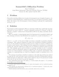
1 Problem
Unipolar Induction
via a Rotating Magnetized Sphere
Kirk T. McDonald
Joseph Henry Laboratories, Princeton University, Princeton, NJ 08544
(November 13, 2012)
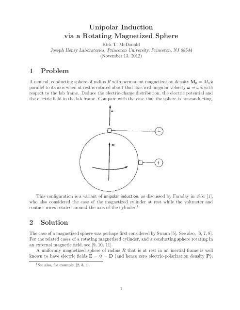
A neutral, conducting sphere of radius R with permanent magnetization density M 0 = M 0 ẑ
parallel to its axis when at rest is rotated about that axis with angular velocity ω = ω ẑ with
respect to the lab frame. Deduce the electric-charge distribution, the electric potential and
the electric field in the lab frame. Compare with the case that the sphere is nonconducting.
This configuration is a variant of unipolar induction, as discussed by Faraday in 1851 [1],
who also considered the case of the magnetized cylinder at rest while the voltmeter and
contact wires rotated around the axis of the cylinder. 1
2 Solution
The case of a magnetized sphere was perhaps first considered by Swann [5]. See also, [6, 7, 8].
For the related cases of a rotating magnetized cylinder, and a conducting sphere rotating in
an external magnetic field, see [9, 10, 11].
A uniformly magnetized sphere of radius R that is at rest in an inertial frame is well
known to have electric fields E =0=D (and hence zero electric-polarization density P),
1 See also, for example, [2, 3, 4].
1

while the magnetic fields are given (in Gaussian units) by
B(r >R)=H(r >R)= 3(m 0 · ˆr)ˆr − m 0
,
r 3 B(r

Likewise, there is a bound surface-charge density,
σ bound (r = R) =P(R − ) · ˆr = ωRM 0 sin 2 θ
, (8)
c
where θ is the polar angle with respect to the z-axis. The total bound charge is zero,
∫
Q bound =
∫
ρ bound dVol+
2.1 Nonconducting Sphere
∫
σ bound dArea = − 8πR3 ωM 0
+ 2πR3 ωM 1 0
(1−cos 2 θ) d cos θ =0.
3c c −1
(9)
If the sphere is nonconducting there are no free charges or currents.
The electric field E can be deduced from a scalar potential V ,
E = −∇V = −∇V ρ − ∇V σ , (10)
where the potential V ρ (continuous at r = R) due to the bound volume-charge density (7) is
V ρ (rR)=− 8πR3 ωM 0
, (11)
3c
3cr
and the potential V σ (also continuous at r = R, andwhichobeys∇ 2 V σ = 0 except at r = R)
due to the bound surface-charge density (8) can be written in the form
V σ (rR)= ∑ n
where P n is the Legendre polynomial of order n. Notingthat
P 0 =1, and P 2 = 3cos2 θ − 1
2
A n
R n+1
r n+1 P n(cos θ), (12)
=1− 3sin2 θ
2
the bound surface-charge density (8) is related to the potential V σ by
σ bound = ωRM 0 sin 2 θ
= 2ωRM 0
c
3c
= E σ,r(R + ) − E σ,r (R − )
4π
(P 0 − P 2 )
( ∂Vσ (R − )
= 1
4π
∂r
− ∂V σ(R + )
)
∂r
, (13)
= ∑ (2n +1) A n
n 4πR P n. (14)
Hence, the Fourier coefficients A n are all zero except that
Thus,
V σ (rR)= 8πωM 0
3c
3
. (15)
( )
R
3
r − R5
5r P 3 2
. (16)

and the total electric potential is
V (r R)=− 4πR5 ωM 0
(3 cos 2 θ − 1).
5c
15cr 3 (17)
The difference ΔV in potential between points on the equator and on the “north” pole of
the sphere is
ΔV = V (θ =90 ◦ ) − V (θ =0)= 4πR2 ωM 0
. (18)
5c
Note also that inside the sphere, V (r R), while inside it 3
D r (r

electric field E are the same as for a conducting sphere, with zero magnetization, that rotates
in a uniform, external magnetic field [11].
The free charges inside the sphere must be at rest relative to the rotating sphere. That
is, the electric field in the comoving frame must be zero at points inside the sphere; E ⋆ =
0=E + v/c × B, recalling eq. (3), so the lab-frame electric field for rR)=− 8πR5 ωM 0
P
3cr 4 2 (cos θ), E θ (r>R)=− 4πR5 ωM 0
sin 2θ. (29)
3cr 4
The difference ΔV in potential between points on the equator and on the “north” pole of
the sphere is
ΔV = V (θ =90 ◦ ) − V (θ =0)= 4πR2 ωM 0
, (30)
3c
which is slightly larger that the result (18) for a nonconducting sphere. Of course, a rotating
nonconducting sphere could not be used as a unipolar generator.
5

For completeness, we note that the surface-charge density is given by
σ total = E r(R + ) − E r (R − )
4π
= 8πRωM 0
[2 − 5P 2 (cos θ)], (31)
9c
of which the bound surface charge is given by eq. (8). Finally, the electric-displacement field
D inside the conducting, magnetized sphere is
2.3 Comments
D(r

[7] L. Davis, Stellar Electromagnetic Fields, Phys.Rev.47, 632 (1947),
http://puhep1.princeton.edu/~mcdonald/examples/EM/davis_pr_72_632_47.pdf
[8] A.I. Miller, Unipolar Induction: A Case Study in the Interaction between Science and
Technology, Ann. Sci. 38, 155 (1981),
http://puhep1.princeton.edu/~mcdonald/examples/EM/miller_as_38_155_81.pdf
[9] K.T. McDonald, Unipolar Induction via a Rotating Magnetized Cylinder (Aug. 17,
2008), http://puhep1.princeton.edu/~mcdonald/examples/magcylinder.pdf
[10] J.J. Thomson, Recent Researches in Electricity and Magnetism (Clarendon Press, 1893),
secs. 434-440,
http://puhep1.princeton.edu/~mcdonald/examples/EM/thomson_recent_researches_sec_434-440.pdf
[11] K.T. McDonald, Conducting Sphere That Rotates in a Uniform Magnetic Field (Mar.
13, 2002), http://puhep1.princeton.edu/~mcdonald/examples/rotatingsphere.pdf
[12] J.D. Jackson, Classical Electrodynamics, 2nd ed. (Wiley, New York, 1975), sec. 5.10.
[13] H. Minkowski, Die Grundgleichen für die elektromagnetischen Vorlage in bewegten
Körpern, Göttinger Nachricthen, pp. 55-116 (1908),
http://puhep1.princeton.edu/~mcdonald/examples/EM/minkowski_ngwg_53_08.pdf
http://puhep1.princeton.edu/~mcdonald/examples/EM/minkowski_ngwg_53_08_english.pdf
[14] J. van Bladel, Relativistic Theory of Rotating Disks, Proc. IEEE 61, 260 (1973),
http://puhep1.princeton.edu/~mcdonald/examples/EM/vanbladel_pieee_61_260_73.pdf
[15] T. Shiozawa, Phenomenological and Electron-Theoretical Study of the Electrodynamics
of Rotating Systems, Proc. IEEE 61, 1694 (1973),
http://puhep1.princeton.edu/~mcdonald/examples/EM/shiozawa_pieee_61_1694_73.pdf
[16] K.T. McDonald, Electrodynamics of Rotating Systems (Aug. 6, 2008),
http://puhep1.princeton.edu/~mcdonald/examples/rotatingEM.pdf
[17] H.A. Lorentz, Alte und Neue Fragen der Physik, Phys.Z.11, 1234 (1910),
http://puhep1.princeton.edu/~mcdonald/examples/EM/lorentz_pz_11_1234_10.pdf
[18] V. Hnizdo and K.T. McDonald, Fields and Moments of a Moving Electric Dipole (Nov.
29, 2011), http://puhep1.princeton.edu/~mcdonald/examples/movingdipole.pdf
[19] S.J. Barnett, Magnetization by Rotation, Phys.Rev.6, 239 (1915),
http://puhep1.princeton.edu/~mcdonald/examples/EM/barnett_pr_6_239_15.pdf
7