Ph501 Electrodynamics Problem Set 1 - Princeton University

Princeton University
Ph501
Electrodynamics
Problem Set 1
Kirk T. McDonald
(1998)
kirkmcd@princeton.edu
http://puhep1.princeton.edu/~mcdonald/examples/
References:
R. Becker, Electromagnetic Fields and Interactions (Dover Publications, New York, 1982).
D.J. Griffiths, Introductions to Electrodynamics, 3rd ed. (Prentice Hall, Upper Saddle
River, NJ, 1999).
J.D. Jackson, Classical Electrodynamics, 3rd ed. (Wiley, New York, 1999).
The classic is, of course:
J.C. Maxwell, A Treatise on Electricity and Magnetism (Dover, New York, 1954).
For greater detail:
L.D. Landau and E.M. Lifshitz, Classical Theory of Fields, 4th ed. (Butterworth-
Heineman, Oxford, 1975); Electrodynamics of Continuous Media, 2nd ed. (Butterworth-
Heineman, Oxford, 1984).
N.N. Lebedev, I.P. Skalskaya and Y.S. Ulfand, Worked Problems in Applied Mathematics
(Dover, New York, 1979).
W.R. Smythe, Static and Dynamic Electricity, 3rd ed. (McGraw-Hill, New York, 1968).
J.A. Stratton, Electromagnetic Theory (McGraw-Hill, New York, 1941).
Excellent introductions:
R.P. Feynman, R.B. Leighton and M. Sands, The Feynman Lectures on Physics, Vol.2
(Addison-Wesely, Reading, MA, 1964).
E.M. Purcell, Electricity and Magnetism, 2nd ed. (McGraw-Hill, New York, 1984).
History:
B.J. Hunt, The Maxwellians (Cornell U Press, Ithaca, 1991).
E. Whittaker, A History of the Theories of Aether and Electricity (Dover, New York,
1989).
Online E&M Courses:
http://www.ece.rutgers.edu/~orfanidi/ewa/
http://farside.ph.utexas.edu/teaching/jk1/jk1.html

Princeton University 1998 Ph501 Set 1, Problem 1 1
1. (a) Show that the mean value of the potential over a spherical surface is equal to the
potential at the center, provided that no charge is contained within the sphere.
(A related result is that the mean value of the electric field over the volume of a
charge-free sphere is equal to the value of the field at its center.)
(b) Demonstrate Earnshaw’s theorem: A charge cannot be held at equilibrium solely
by an electrostatic field. 1
(c) Demonstrate that an electrostatic field E cannot have a local maximum of E 2 ,
using the mean value theorem mentioned in part (a) – or any other technique.
Remark: An interesting example of nonelectrostatic equilibrium is laser trapping
of atoms. Briefly, an atom of polarizability α takes on an induced dipole moment
p = αE in an electric field. The force on this dipole is then (Notes, p. 26),
F = ∇(p · E) =α∇E 2 . Since an electrostatic field cannot have a local maximum
of E 2 , it cannot trap a polarizable atom. But consider an oscillatory field, in
particular a focused light wave. The time-average force, 〈F〉 = α∇ 〈E 2 〉 draws
the atom into the laser focus where the electric field is a maximum. See,
http://puhep1.princeton.edu/~mcdonald/examples/tweezers.pdf
1 http://puhep1.princeton.edu/~mcdonald/examples/EM/earnshaw_tcps_7_97_39.pdf

Princeton University 1998 Ph501 Set 1, Problem 2 2
2. Calculate the potential φ(z) along the axis of a disk of radius R in two cases:
(a) The disk is a uniform layer of charge density σ, and
(b) The disk is a uniform dipole layer of dipole moment density p = pẑ per unit area.

Princeton University 1998 Ph501 Set 1, Problem 3 3
3. Suppose the electric field of point charge q were E = qˆr/r 2+δ where δ ≪ 1, rather then
E = qˆr/r 2 .
(a) Calculate ∇ · E and ∇ × E for r ≠ 0. Find the electric potential for such a point
charge.
(b) Two concentric spherical conducting shells of radii a and b are joined by a thin
conducting wire. Show that if charge Q a resides on the outer shell, then the charge
on the inner shell is
Q b ≃−
Q aδ
[2b ln 2a − (a + b)ln(a + b)+(a − b)ln(a − b)] (1)
2(a − b)

Princeton University 1998 Ph501 Set 1, Problem 4 4
4. (a) Starting from the dipole potential φ = p · r/r 3 explicitly show that
E =
3(p · ˆr)ˆr − p
r 3
− 4πp
3 δ3 (r). (2)
Hint: to show the need for the δ 3 (r) term, consider the volume integral of E over
a small sphere about the dipole. You may need a variation of Gauss’ theorem:
∫
∮
∇φ dVol = φˆn dS, (3)
V
where ˆn is the outward normal to the surface.
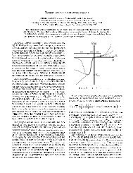
(b) The geometric definition of the “lines of force” is that this family of curves obeys
the differential equation:
dx
= dy = dz . (4)
E x E y E z
For a dipole p = pẑ, find the equation of the lines of force in the x-z plane. It is
easiest to work in spherical coordinates. Compare with the figure on the cover of
the book by Becker.
S

Princeton University 1998 Ph501 Set 1, Problem 5 5
5. Find the two lowest-order nonvanishing terms in the multipole expansion of the potential
due to a uniformly charged ring of radius a carrying total charge Q. Takethe
origin at the center of the ring, and neglect the thickness of the ring.

Princeton University 1998 Ph501 Set 1, Problem 6 6
6. (a) A long, very thin rod of dielectric constant ɛ is oriented parallel to a uniform
electric field E ext .WhatareE and D inside the rod?
(b) What are E and D inside a very thin disc of dielectric constant ɛ if the disc is
perpendicular to E ext ?
(c) Find E and D everywhere due to a sphere of fixed uniform polarization density
P. Thencalculate ∫ E·D dVol for the two volumes inside and outside the sphere’s
surface.
Hint: this problem is equivalent to two oppositely charged spheres slightly displaced.
(d) Show that for any finite electret, a material with fixed polarization P,
∫
all space
E · D dVol = 0. (5)

Princeton University 1998 Ph501 Set 1, Problem 7 7
7. A spherical capacitor consists of two concentric conducting shells of radii a and b.
The gap is half filled with a (non-conducting) dielectric liquid of constant ɛ. Youmay
assume the fields are radial. The inner shell carries charge +Q, the outer shell −Q.
Calculate E and D in the gap, and the charge distribution in the inner shell. Also
calculate the capacitance, defined as C = Q/V ,whereV is the potential difference
between the inner and outer shells.

Princeton University 1998 Ph501 Set 1, Problem 8 8
8. (a) As a classical model for atomic polarization, consider an atom consisting of a fixed
nucleus of charge +e with an electron of charge −e in a circular orbit of radius a
about the nucleus. An electric field is applied at right angles to the plane of the
orbit. Show that the polarizability α is approximately a 3 . (This happens to be
the result of Becker’s (26-6), but the model is quite different!)
Assuming that radius a is the Bohr radius, ∼ 5.3 × 10 −9 cm, use the model
to estimate the dielectric constant ɛ of hydrogen gas at S.T.P. Empirically, ɛ ∼
1+2.5 × 10 −4 .
(b) Another popular classical model of an atom is that the electron is bound to a
neutral nucleus by a spring whose natural frequency of vibration is that of some
characteristic spectral line. For hydrogen, a plausible choice is the Lyman line at
1225 Angstroms. In this model, show that α = e 2 /mω 2 , and estimate ɛ. Recall
that e =4.8 × 10 −10 esu, and m =9.1 × 10 −28 g.

Princeton University 1998 Ph501 Set 1, Solution 1 9
Solutions
1. a) We offer two solutions: the first begins by showing the result holds for small spheres,
and then shows the result is independent of the size of the (charge-free) sphere; the
second applies immediately for spheres of any size, but is more abstract.
We consider a charge-free sphere of radius R centered on the origin.
In a charge-free region, the potential φ(r) satisfies Laplace’s equation:
∇ 2 φ =0. (6)
First, we simply expand the potential in a Taylor series about the origin:
φ(r) =φ(0) + ∑ i
∂φ(0)
x i + 1 ∑ ∂ 2 φ(0)
x i x j + ... (7)
∂x i 2
i,j
∂x i ∂x j
We integrate (7) over the surface of the sphere:
∮
φ(r)dS =4πR 2 φ(0) + ∑ ∂φ(0)
x i dS +
S
i
∂x i
∮S 1 ∑ ∂ 2 φ(0)
x i x j dS + ... (8)
2
i,j
∂x i ∂x j
∮S
For a very small sphere, we can ignore all terms except the first, In this case, eq. (8)
becomes
1
φ(r)dS = φ(0), [R “small”], (9)
4πR 2 ∮S
which was to be shown.
Does the result still hold at larger radii? One might expect that since “small” is not
well defined, (9) holds for arbitrary R, so long as the sphere is charge free.
Progress can be made staying with the Taylor expansion. By spherical symmetry, the
integral of the product of an odd number of x i vanishes. Hence, only the terms with
even derivatives of the potential survive. And of these, only some terms survive. In
particular, for the 2nd derivative, only the integrals of x 2 1, x 2 2,andx 2 3 survive, and these
3 are all equal. Thus, the 2nd derivative term consists of
(
1 ∂ 2 ) ∮
φ(0)
+ ∂2 φ(0)
+ ∂2 φ(0)
x 2
2 ∂x 2 1 ∂x 2 2 ∂x
1dS, (10)
2
3 S
which vanishes, since ∇ 2 φ(0) = 0.
It is less evident that the terms with 4rth and higher even derivatives vanish, although
this can be shown via a systematic multipole expansion in spherical coordinates, which
emphasizes the spherical harmonics Yl m .
But by a different approach, we can show that the mean value of the potential over a
charge-free sphere is independent of the radius of the sphere. That is, consider
M(r) = 1 φdS =
4πr
∮S
1 ∫
2 4π
∫
d cos θ
dϕφ(r, θ, ϕ), (11)

Princeton University 1998 Ph501 Set 1, Solution 1 10
in spherical coordinates (r, θ, ϕ). Then
dM(r)
dr
= 1 ∫
4π
1
=
4πr 2 ∮S
∫
d cos θ
dϕ ∂φ
∂r = 1 ∫
4π
∫
d cos θ
dϕ∇φ · ˆr
∇φ · dS = 1 ∇
4πr
∫V
2 φdVol = 0, (12)
2
for a charge-free volume. Hence, the mean value of the potential over a charge-free
sphere of finite radius is the same as that over a tiny sphere about the center of the
larger sphere. But, as shown in the argument leading up to (9), this is just the value
of the potential at the center of the sphere.
A second solution is based on one of Green’s theorems (sec. 1.8 Of Jackson). Namely,
for two reasonable functions φ(r) andψ(r),
∫
V
(
φ∇ 2 ψ − ψ∇ 2 φ ) ∮
dVol =
S
(
φ ∂ψ
∂n − ψ ∂φ )
dS, (13)
∂n
where n is coordinate normally outward from the closed surface S surrounding a volume
V .
With φ as the potential satisfying Laplace’s equation (6), the second term on the l.h.s.
of (13) vanishes. We seek an auxiliary function ψ such that ∇ 2 ψ = δ 3 (0), so the l.h.s.
is just φ(0). Further, it will be helpful if ψ vanishes on the surface of the sphere of
radius R, so the second term on the r.h.s. vanishes also.
These conditions are arranged with the choice
ψ = 1 ( 1
4π R − 1 )
, (14)
r
recalling pp. 8-9 of the Notes. On the surface of the sphere, coordinate n is just the
radial coordinate r, so
∂ψ
∂n = 1
4πr . (15)
2
Thus, we can evaluate the expression (13), and get:
ψ(0) = 1 φdS, (16)
4πR
∮S
2
which means that the value of the potential φ at the center of a charge-free sphere of
any size is the average of the potential on the surface of the sphere.
b) The potential energy of a charge q at point r, due to interaction with an electrostatic
field derivable from a potential φ(r), is:
U = qφ(r). (17)
For the point r 0 to be the equilibrium point for a particle, the potential φ should have
a minimum there. But we can infer from part (a) that:

Princeton University 1998 Ph501 Set 1, Solution 1 11
Harmonic functions do not have minima,
harmonic functions being a name for solutions of Laplace’s equation (6).
Indeed, a minimum of U at point r 0 would imply that there is a small sphere centered
on r 0 such that φ(r 0 )islessthanφ at any point on that sphere. This would contradict
what we have shown in part (a): φ(r 0 ) is the average of φ over the sphere.
We continue with an example of Earnshaw’s theorem. Consider 8 unit charges located
at the corners of a cube of edge length 2, i.e., the charges are at the locations (x i ,y i ,z i )
= (1,1,1), (1,1,-1), (1,-1,1), (1,-1, -1), (-1,1,1), (-1,1,-1), (-1,-1,1), (-1,-1,1). It is suggestive,
but not true, that the electric field near the origin points inwards and could
trap a positive charge.
The symmetry of the problem is such that a series expansion of the electric potential
near the origin will have terms with only even powers, and we must go to 4rth order to
see that the potential does not have a maximum at the origin. To simplify the series
expansion, we consider the electric field, for which we need expand only to third order.
The electric potential is given by
φ =
8∑
i=1
The x component of the electric field is
1
√(x i − x) 2 +(y i − y) 2 +(z i − z) 2 . (18)
E x = − ∂φ 8∑
∂x = − x i − x
[(x i − x) 2 +(y i − y) 2 +(z i − z) 2 ] 3/2
i=1
= − 1 8∑
x i − x
3 3/2 i=1
[1 + (−2x i x − 2y i y − 2z i z + x 2 + y 2 + z 2 )/3] 3/2
≈ − 1 [
8∑
x
3 3/2 i 1+y i y + z i z + −2x2 + y 2 + z 2 ]
+5y i yz i z
i=1
3
− 1 [
8∑ 11yi y 3 +11z i z 3
x
3 3/2 i − x2 y i y + x 2 z i z
+ 3y2 z i z +3z 2 ]
y i y
i=1
54
6
2
− 1
[
8∑ 2xyi y +2xz i z
− 7x3
3 3/2 i=1
3 54 + 7xy2 +7xz 2
+ 20xy ]
iyz i z
6
9
28
=
81 √ 3 (x3 − 9xy 2 − 9xz 2 ), (19)
noting that x 2 i = yi 2 = zi 2 =1andthat ∑ x i =0= ∑ x i y i , etc. Similarly,
E y ≈ 28
81 √ 3 (y3 − 9yx 2 − 9yz 2 ) and E z ≈ 28
81 √ 3 (z3 − 9zx 2 − 9zy 2 ). (20)
The radial component of the electric field is therefore
E r = E · r
r
= xE x + yE y + zE z
r
≈ 28
81 √ 3r [x4 + y 4 + z 4 − 18(x 2 y 2 + y 2 z 2 + z 2 x 2 )]. (21)

Princeton University 1998 Ph501 Set 1, Solution 1 12
Along the x axis, r = x and the radial field varies like
but along the diagonal x = y = z = r/ √ 3 it varies like
E r ≈ 28
81 √ 3 r3 > 0, (22)
E r ≈− 476
243 √ 3 r3 < 0. (23)
It is perhaps not intuitive that the electric field is positive along the positive x axis,
although Earnshaw assures us that the radial electric field must be positive in some
direction. A clue is to consider the point (1,0,0) on the face of the cube whose corners
hold the charges. At this point the electric fields due to the 4 charges with x =1sum
to zero, so the field here is due only to the 4 charges with x = −1, and now “obviously”
the x component of the electric field is positive. The charges at the corners of the cube
force a positive charge toward the origin along the diagonals, but cannot prevent that
charge from escaping near the centers of the faces of the cube.
c) If E 2 has a local maximum at some point P in a charge-free region, then there is a
nonzero r such that E 2

Princeton University 1998 Ph501 Set 1, Solution 2 13
2. a) The potential φ(z) along the axis of a disk of radius R of charge density σ (per unit
area) is given by the integral:
φ(z) =
∫ R
r=0
σ
2πrdr√ r2 + z =2πσ ( √
R2 + z 2 −|z| ) . (26)
2
Notice that φ(z) behaves as πσR 2 /|z| for |z| ≫R, which is consistent with the observation
that in this limit the disk may be considered as a point charge q = πσR 2 .
Notice also, that at z = 0 the potential is continuous, but it’s first derivative (−E)
jumps from −2πσ at z =0 + to 2πσ at z =0 − . This reflects the fact that at small |z|
(|z| ≪R) the potential may be calculated, in first approximation, as the potential for
the infinite plane with charge density σ.
b) A disk of dipole-moment density p = pẑ can be thought of as composed of a layer
of charge density +σ separated in z from a layer of charge density −σ by a distance
d = p/σ. Say, the + layer is at z = d/2, and the − layer is as z = −d/2. Then, the
potential φ b at distance z along the axis could be written in terms of φ a (z) found in
(26) as
φ b (z) =φ a (z − d/2) − φ a (z + d/2) →−d ∂φ a(z)
∂z
=2πp
(
sign(z) −
)
z
√ . (27)
R2 + z 2
In this, we have taken the limit as d → 0 while σ →∞, but p = σd is held constant.
At large z we get the potential of a dipole P = πpR 2 on its axis. But near the plate
(|z| ≪R), the potential has a discontinuity:
φ b (0 + ) − φ b (0 − )=4πp. (28)
We may explain this in our model of the dipole layer as a system of two close plates
with charge density σ and distance d between them, where p = σd. The field between
the plates is E z = −4πσ, and the potential difference potential between two plates is
as found in (28).
Δφ = −E z d =4πp, (29)

Princeton University 1998 Ph501 Set 1, Solution 3 14
3. a) For a charge q at the origin, the proposed electric field is
E = q ˆr
r = q r . (30)
2+δ r3+δ This still has spherical symmetry, so we can easily evaluate the divergence and curl in
spherical coordinates:
∇ · E = q ∇ · r 1
+ qr · ∇
r3+δ r = 3q 3+δ
− q = − qδ ; (31)
3+δ r3+δ r 3+δ r3+δ ∇ × E = q ∇ × r + ∇ 1
r
× qr =0− (3 + δ) × qr =0. (32)
r 3+δ r3+δ r5+δ Since ∇ × E = 0, the field can be derived from a potential. Indeed,
∫ r
E = −∇φ, where φ = −
∞
∫ r
E r dr = −q
∞
dr
r 2+δ = 1
q
. (33)
δ +1rδ+1 b) Let us first compute the potential due to a the spherical shell of radius a that carries
charge Q, as observed at a distance r from the center of the sphere. We use (33) and
integrate in spherical coordinates (r, θ, φ) to find
φ(r) =
Q
4πa 2 1
1+δ
∫ 1
−1
2πar 2 d cos θ
(a 2 + r 2 − 2ar cos θ) 1+δ
2
= Q (a + r) 1−δ −|a − r| 1−δ
2ar 1 − δ 2 . (34)
Now consider the addition of a sphere of radius b

Princeton University 1998 Ph501 Set 1, Solution 4 15
4. a) The first terms in E can be obtained by explicit differentiation, perhaps best done
using vector components. For r>0,
E i = − ∂ p j x j
∂x i r 3
= 3(p jx j )x i
r 5
− p i
r 3 . (40)
To justify the δ-term, consider the integral over a small sphere surrounding the (point)
dipole:
∫
∫
∮
∮
p · r
EdVol = − ∇φdVol = φˆndS = ˆrdS, (41)
V
V
S
S r3 according to the form of Gauss’ law (3) given in the hint. Evaluating the last integral in
a spherical coordinate system with z axis along p, we find that only the ˆp component
is nonzero:
∫
∫ 1
EdVol = p
−1
2πdcos θ cos 2 θ = 4πp
3 . (42)
No matter how small the sphere, the integral (42) remains the same.
On the other hand, if we insert the field E from (40) in the volume integral, only the
z component (along p) does not immediately vanish, but then
∫
V
E z dVol =
∫ r
0
2πrdr
∫ 1
−1
d cos θ p(3 cos2 θ − 1)
r 3 =0, (43)
if we adopt the convention that the angular integral is performed first.
To reconcile the results (42) and (43), we write that the dipole field has a spike near
the origin symbolized by −(4πp/3)δ 3 (r).
Another qualitative reason for the δ-term is as follows. Notice, that without this term
we would conclude that the electric field on the axis of the dipole (z-axis) would always
along +z. This would imply that if we moved some distribution of charge from large
negative z to large positive z, then that charge would gain energy from the dipole
field. But this cannot be true: after all, the dipole may be thought as a system of two
charges, separated by a small distance, and for such a configuration the potential at
large distances is certainly extremely small.
We can also say that the δ-term, which points in the −p direction, represents the large
field in the small region between two charges that make up the dipole.
b) In spherical coordinates with ẑ along p, the dipole potential in the x-z plane is
Then,
E r = − ∂φ
∂r
φ(r, θ) = p cos θ
r 2 (44)
=
2p cos θ
r 3 , and E θ = − ∂φ
r∂θ = p sin θ
r 3 . (45)

Princeton University 1998 Ph501 Set 1, Solution 4 16
Thus, the differential equation of the field lines
dr
E r
= rdθ
E θ
,
implies
dr
r
=2d
sin θ
sin θ , (46)
which integrates to
etc.
r = C sin 2 θ = C x2
r 2 , (47)

Princeton University 1998 Ph501 Set 1, Solution 5 17
5. The multipole expansion of the potential φ about the origin due to a localized charge
distribution ρ(r) is
φ(r) = Q r + P · ˆr + 1 Q ijˆr iˆr j
+ ... (48)
r 2 2 r 3
where
∫
∫
∫
Q = ρ(r)dVol, P i = ρr i dVol, Q ij = ρ(3r i r j − δ ij r 2 )dVol, ... (49)
For the ring, Q is just the total charge, while the dipole moment P is zero because of
the symmetry.
Let us find the quadrupole moment, Q ij .Takethez axis to be along that of the ring.
Then, the quadrupole tensor is diagonal, and due to the rotational invariance,
We compute Q xx in spherical coordinates (r, θ, ϕ):
Q xx = Q yy = − 1 2 Q zz. (50)
∫
Q xx =
ρ(3x 2 − r 2 )dVol =
∫ 2π
0
Q
2πa a2 (3 cos 2 ϕ − 1)adϕ = Qa2
2 . (51)
Thus, the third term in the expansion (48) is:
1
2r 3 (
Qxx sin 2 θ cos 2 ϕ + Q yy sin 2 θ sin 2 ϕ + Q zz cos 2 θ ) = − Qa2
4r 3 (3 cos2 θ − 1). (52)

Princeton University 1998 Ph501 Set 1, Solution 6 18
6. a) Remember that E is defined as a mean electric field, due to both the external field
and the microscopic charges.
In the presence of external field E ext , polarization P is induced in the rod. Since
∇ × E = 0, the tangential electric field is continuous across the surface of the rod.
This suggests that inside the rod, which is parallel to E ext ,wehaveE = E ext .
To check for consistency, note that in this case, P is constant apart from the ends.
There is no net polarization charge in the bulk of the rod, and no change in the electric
field from E ext . But at the ends there are charges ±Q, whereQ = PA,andA is
the cross-sectional area of the rod. Since A is very small for the thin rod, and the
ends of a long rod are far away from most of the rod, these charges do not contribute
significantly to the electric field. Hence our hypothesis is satisfactory.
The electric displacement can then be deduced as D = ɛE = ɛE ext inside the rod.
b) For a dielectric disk perpendicular to E ext , the normal component of the fields is
naturally emphasized. Recall that ∇ · D implies that the normal component of the
displacement D is continuous across the dielectric boundary.
Outside the disk, where ɛ =1,D = E = E ext is normal to the surface. (That E = E ext
may be justified by noting that the induced charges on two surfaces of the thin disk
have opposite signs and do not contribute to the field outside of the disk.) Thus, inside
the disk, D = E ext . Lastly, inside the disk E = D/ɛ = E ext /ɛ.
c) The problem of a dielectric sphere of uniform polarization density P is equivalent
to two homogeneous spheres with charge densities ρ and −ρ, displaced by distance d,
such that in the limit d → 0, ρ →∞but ρd = P.
Recall that for a sphere of uniform charge density ρ, the interior electric field is
E = 4π 3
ρr. (53)
Thus, inside the polarized sphere we have
{ 4π
E = lim
3 ρ(r − d) − 4π }
3 ρr = − 4π 3
The displacement is
Then,
∫
inside
lim ρd = −4πP
3 . (54)
D = E +4πP = 8πP
3 . (55)
E · DdVol = − 4πP
3
8πP
3
4πr 3
3
= − 128π2 r 3 P 2
. (56)
27
Outside the sphere, the electric field is effectively due to two point charges q =4πρr 3 /3
separated by small distance d, whereρd = P. The external field is simply that of a
point dipole at the origin of strength
p = 4πr3 P
. (57)
3

Princeton University 1998 Ph501 Set 1, Solution 6 19
Then,
and D = E. Thus,
∫
outside
∫
= p 2 ∞
r
E · DdVol =
4πr 2 dr
r 6
∫∞
+3p 2
E =
3ˆr(p · ˆr) − p
r 3 , (58)
∫ p 2 +3(p · ˆr) 2 )
r 6 dVol (59)
r
2πr 2 ∫1
dr
r 6
−1
cos 2 θdcos θ = 8πp2 = 128π3 r 3 P 2
,
3r 3 27
and the sum of the inside and outside integrals vanishes.
d) Let us show, on general grounds, that for an electret the integral of E · D over the
whole space is zero. First, note that ∇ · D = 0 everywhere for an electret, and that
the electric field can be derived from a potential, φ. Then
∫
all space
∫
∫
∮
E · DdVol = − ∇φ · DdVol = − ∇ · (φD)dVol = − φD · dS. (60)
V
V
S
But if electret occupies finite volume, then φ ≃ 1/r at large r, as seen from multipole
expansion; in the same limit, D ≃ 1/r 2 , while dS ≃ r 2 . So the integral over the surface
at infinity is zero.
What would be different in this argument if the material were not an electret? In
general, we would then have ∇ · D =4πρ free , and the 3rd step in (60) would have the
additional term ∫ V φ∇ · D =4π ∫ V ρ freeφ =8πU. Thus, the usual electrostatic energy
is contained in ∫ V E · D/8π, as expected.
This argument emphasizes that the work done in putting a field on an ordinary dielectric
can be accounted for using only the free charges (which establish D). One
need not explicitly calculate the energy stored in the polarization charge distribution,
which energy is accounted for via the modification to the potential φ in the presence
of the dielectric. But the whole argument fails for an electret, which remains polarized
(energized) even in the absence of a free charge distribution.

Princeton University 1998 Ph501 Set 1, Solution 7 20
7. In the upper half of the capacitor (where there is no dielectric) we have via Gauss’ law:
E up (r) =D up (r) = 4πQ up
2πr 2
= 2Q up
r 2 , (61)
where Q up is the charge on the upper half of the inner sphere, assuming the fields are
radial.
In the lower part we have:
E down (r) =E up (r), (62)
which follows from the continuity of the tangential component of E across the boundary
between dielectric and vacuum. Also,
D down (r) =ɛE down (r), (63)
and
D down (r) = 2Q down
, (64)
r 2
as follows from ∇ · D =4πρ free ,whereQ down is the charge on the lower part of the
inner sphere.
Combining (61-64),
Q down = ɛQ up , (65)
holds for the “free” charge on the inner shell.
What about the total charge distribution, which include polarization charges in the
dielectric? The polarization vector P obeys 4πP =(ɛ − 1)E. Thus, the charge density,
σ =4πP · ˆn, which appears microscopically on the boundary of the dielectric adjacent
to the inner shell, equals 1 − ɛ times the charge density on the upper shell (since
ˆn = −ˆr). In other words, the total microscopic charge densities on the lower and
upper parts of the shell are equal. This ensures that the electric field is the same in
the upper and lower part of the capacitor.
Of course,
Q down = Q − Q up . (66)
From (65) and (67),
Q − Q up = ɛQ up , (67)
and hence,
Q up =
Q
1+ɛ . (68)
This implies that the potential difference V between the shells is
So, the capacitance is
∫b
V = −
a
Edr = − 2Q ∫b
dr
1+ɛ r = 2 a
C = Q V = 1+ɛ
2
2Q [ 1
1+ɛ b − 1 ]
. (69)
a
ab
a − b . (70)

Princeton University 1998 Ph501 Set 1, Solution 8 21
8. a) In the presence of an electric field along the z direction, which is perpendicular to
the plane of the orbit of our model atom, the plane is displaced by a distance z. We
calculate this displacement from the equilibrium condition: the axial component of the
Coulomb force between the electron and the proton should be equal to the force eE
on the electron of charge e due to the electric field. Namely,
F z = e2 z
= eE, (71)
r 2 r
where r = √ a 2 + z 2 ,anda is the radius of the orbit of the electron. The induced
atomic dipole moment p is
p = ez = r 3 E ≈ a 3 E, (72)
where the approximation holds for small displacements, i.e., small electric fields. Since
p = αE in terms of the atomic polarizability α, weestimatethat
α ≈ a 3 , (73)
where a is the radius of the atom.
The dielectric constant ɛ is related to the atomic polarizability via
ɛ − 1=4πNα, (74)
where N is the number of atoms per cm 3 . For hydrogen, there are 2 atoms per molecule,
and 6 × 10 23 molecules in 22.4 liters, at S.T.P. Hence N =2(6× 10 23 )/(22.4 × 10 3 )=
5.4 × 10 19 atoms/cm 3 . Estimating the radius a as the Bohr radius, 5.3 × 10 −9 cm, we
find
ɛ − 1 ≈ 4π(5.4 × 10 19 )(5.3 × 10 −9 ) 3 ≈ 1.0 × 10 −4 . (75)
b) If an electric field E is applied to the springlike atom, then the displacement d of
the electron relative to the fixed (neutral) nucleus is related by F = kd = eE, where
k = mω 2 is the spring constant in terms of characteristic frequency ω. The induced
dipole moment p is given by
p = ed = e2 E
k
Thus the polarizability α is given by
= e2 E
mω 2 . (76)
α =
e2
mω 2 . (77)
The frequency ω that corresponds to the Lyman line at 1225
Ais
ω = 2πc
λ = 2π(3 × 1010 )
1225 × 10 =1.54 × −8 1016 Hz. (78)
From (77),
α =
(4.8 × 10 −10 ) 2
(9.1 × 10 −28 )(1.54 × 10 16 ) 2 =1.07 × 10−24 cm 3 . (79)

Princeton University 1998 Ph501 Set 1, Solution 8 22
Finally,
ɛ − 1=4πNα =4π(5.4 × 10 19 )(1.07 × 10 −24 )=7.3 × 10 −4 (80)
Thus, our two models span the low and high side of the empirical result. Of course,
we have neglected the fact that the hydrogen atoms are actually paired in molecules.