Sommerfeld's Diffraction Problem - Princeton University

1 Problem
Sommerfeld’s Diffraction Problem
Kirk T. McDonald
Joseph Henry Laboratories, Princeton University, Princeton, NJ 08544
(January 22, 2012; updated April 30, 2013)
Discuss the scattering (diffraction) of a plane electromagnetic wave of angular frequency ω by
a perfectly conducting half plane, considering the latter to be the limit of a parabolic cylinder.
Relate the results to the electromagnetic version of Babinet’s principle for complementary
screens [1, 2, 3]. 1
2 Solution
Experiments in which polarization effects in scattering of light from a knife edge were first
performed by Gouy in 1883 [7]. A partial explanation was given by Poincaré in 1892 [8].
This first “complete” solution was by Sommerfeld in 1895 [9, 10], using a somewhat obscure
technique. 2
Here, we consider a conducting knife edge to be a limiting case of a parabolic cylinder, and
take advantage of the fact that Helmholtz wave equation for a scalar wavefunction ψe −iωt ,
(∇ 2 + k 2 )ψ =0, (1)
where k = ω/c and c is the speed of light in vacuum, is separable in parabolic-cylindrical
coordinates. Then, using an expansion of a plane wave in parabolic-cylindrical coordinates
[13, 14, 15], the problem of scattering of a plane wave by a surface of constant coordinates can
be given a series solution. This technique was first employed for scattering by a conducting
cylinder [16], using the expansion of a plane wave in cylindrical coordinates found by Jacobi
[17]. This technique can be used for surfaces of constant coordinate in the 11 coordinate
systems in which the Helmholtz equation is separable [18], and permits formal solutions to
a larger set of electromagnetic scattering problems than is commonly acknowledged. The
example of a conducting strip as a limit of an elliptical cylinder is considered in sec. 3 of
[19].
The relevance of parabolic-cylindrical coordinates to the knife-edge problem was realized
by Lamb [20, 21], who used them to give an alternative derivation of Sommerfeld’s solution,
which alternative we follow here. 3 Other studies related to that of the present note include
[22, 25, 26, 27, 28, 29, 30, 31]. See also the Appendix.
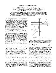
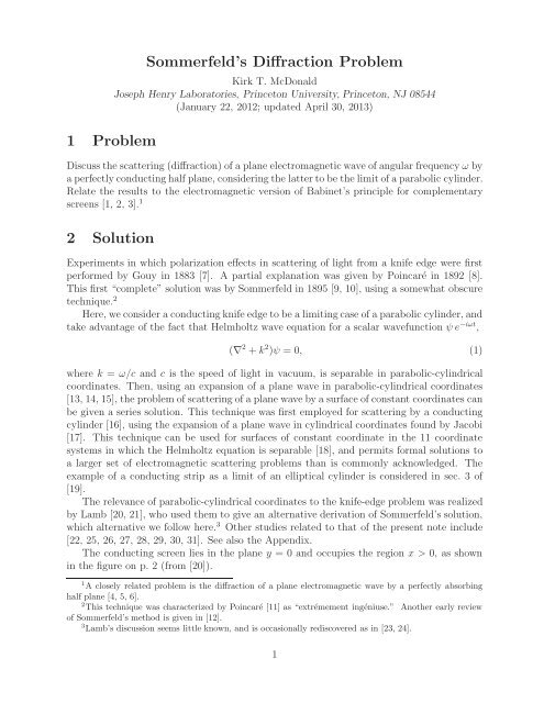
The conducting screen lies in the plane y = 0 and occupies the region x>0, as shown
in the figure on p. 2 (from [20]).
1 A closely related problem is the diffraction of a plane electromagnetic wave by a perfectly absorbing
half plane [4, 5, 6].
2 This technique was characterized by Poincaré [11]as“extrémement ingéniuse.” Another early review
of Sommerfeld’s method is given in [12].
3 Lamb’s discussion seems little known, and is occasionally rediscovered as in [23, 24].
1

In addition to ordinary cylindrical coordinates (r, φ, z), we consider parabolic-cylindrical
coordinates (ξ,η,z) which are related (for 0 ≤ φ ≤ 2π) by
x + iy = re iφ (ξ + iη)2
= ,
2
x = ξ2 − η 2
, y = ξη, (2)
2
ξ = √ 2r cos φ 2 , η = √ 2r sin φ 2 . (3)
In this convention, the sign of ξ at a point (ξ,η) =(x, y) isthesameasthesignofy, while
η is always non-negative. The half plane (x >0,y = 0) corresponds to η =0,andthe
complementary half plane (x

2.1 Normal Incidence
We first consider incident waves of the form e i(ky−ωt) , which are normally incident on the
screen from y

Using the fact,
we have that
a u +
∫ ∞
0
e −iζ2 dζ =
√ π
2 e−iπ/4 , (16)
√ √ π
π
2 b u e −iπ/4 =0, a v −
2 b v e −iπ/4 =0. (17)
Finally, the condition that E z = E 0 e iky + ψ s vanish on the surface of the conducting screen
implies that
∫ √
− E 0 = ψ s (x>0, 0) = ψ s kξ/2
(ξ,0) = a u + a v +(b u + b v ) e −iζ2 dζ, (18)
0
and hence,
Combining this with eq. (64) we find 4
and
ψ s = E s z = E 0
( e
i(ky+π/4)
√ π
a u + a v = −E 0 , b v = −b u . (19)
a u = a v = − E 0
2 , b u = −b v = E 0
√ π
e iπ/4 , (21)
∫ √ k(ξ+η)/2
0
e −iζ2 dζ − e−i(ky−π/4)
√ π
2.1.2 Electric Field Perpendicular to the Edge
∫ √ k(ξ−η)/2
0
e −iζ2 dζ − eiky + e −iky )
.(22)
2
In this case the current on the conducting screen are in the x-direction, so the scattered
electric field lies in the x-y plane, while both the incident and scattered magnetic field are
parallel to the edge. It is therefore convenient to consider the scalar wavefunction ψ = B z =
E 0 e iky + ψ s (x, y).
The analysis for ψ s is similar to the preceding sec. 2.1.1, except that the boundary
condition at the screen, E x (x>0, 0) = 0 implies that ∂B z (x>0, 0)/∂y =0,i.e.,
∂Bz s(x>0, 0)/∂y = ∂Bs z (ξ, 0)/∂y = −ikE 0.
4 In view of eq. (20), and recalling that the sign of ξ is taken to be the same as that of y, wehavethat
∫ √ √
ψ s (x, −y) = a u e −iky + a v e iky + b u e −iky k(−ξ+η)/2
∫ − k(ξ+η)/2
e −iζ2 dζ + b v e iky e −iζ2 dζ
0
∫ k(ξ−η)/2
∫ √
= a v e −iky + a u e iky + b v e −iky e −iζ2 dζ + b u e iky k(ξ+η)/2
e −iζ2 dζ
0
= ψ s (x, y). (20)
That is, ψ s = E s z satisfies the symmetry (6), as expected.
0
0
4

To perform the derivative of the integrals in eq. (14) we need the relations
Using these, we find
∂ψ s (x>0, 0)
∂y
and hence,
∂ξ
∂x = ξ 2r ,
∂ξ
∂y = η 2r ,
= −ikE 0 = ik(a u − a v )+(b u − b v )
Combining this with eq. (64) we find 5
and
ψ s = B s z = E 0
(
e
i(ky+π/4)
√ π
∂η
∂x = − η 2r , (23)
∂η
∂y = ξ 2r . (24)
(
ik
∫ √ kξ/2
0
e −iζ2 dζ +
√ )
k
2ξ e−i√ kξ 2 /2
, (25)
a u − a v = −E 0 , b u = b v . (26)
a u = −a v = − E 0
2 , b u = b v = E 0
√ π
e iπ/4 , (28)
∫ √ k(ξ+η)/2
0
e −iζ2 dζ + e−i(ky−π/4)
√ π
∫ √ k(ξ−η)/2
2.1.3 Asymptotic Behavior near the Geometric Shadow
0
e −iζ2 dζ − eiky − e −iky )
.(29)
2
To exhibit the well-known behavior of the fields near the edge of the geometric shadow (first
deduced by Fresnel in a scalar theory), it is convenient to recast the integrals in eqs. (22)
and (29) as running from ζ to ∞,
ψ s
∫
= − ei(ky+π/4) ∞
∫
√ √ e −iζ2 dζ ± e−i(ky−π/4) ∞
√ √ e −iζ2 dζ ∓ e −iky . (30)
E 0 π k(ξ+η)/2 π k(ξ−η)/2
We consider these waves for large y = ξη ≈ ξ 2 ≈ η 2 and small x =(ξ 2 − η 2 )/2 ≈ (ξ − η)/ √ y,
where the total wavefunction ψ = E 0 e iky + ψ s has the form
∫
ψ
≈± e−i(ky−π/4) ∞√kx ∫
√ e −iζ2 dζ + e iky ∓ e −iky ≈± e−i(ky−π/4) ∞√kx
√ e −iζ2 dζ, (31)
E 0 π 2 /y
π 2 /y
5 In view of eq. (28), and recalling that the sign of ξ is taken to be the same as that of y, wehavethat
∫ √
ψ s (x, −y) = a u e −iky + a v e iky + b u e −iky k(−ξ+η)/2
∫
√
− k(ξ+η)/2
e −iζ2 dζ + b v e iky e −iζ2 dζ
0
∫ √
= −a v e −iky − a u e iky − b v e −iky k(ξ−η)/2
∫ √
e −iζ2 dζ − b u e iky k(ξ+η)/2
e −iζ2 dζ
0
= −ψ s (x, y). (27)
That is, ψ s = B s z satisfies the symmetry (6), as expected.
0
0
5

where the second approximation follows noting that the integral varies more slowly with y
than the terms e iky ∓ e −iky , which can be represented by their average, namely zero. The
real and imaginary parts of the remaining integral are related to the Fresnel cosine and sine
integrals,
√
∫ t
∫ √ √
C(t) = cos πs2 2
0 2 ds = π/2 t
∫ t
∫ √
cos s 2 ds, S(t) = sin πs2 2
π 0
0 2 ds = π/2 t
sin s 2 ds,(32)
π 0
and the integral itself √ has the interpretation √ of the length of the chord on the Cornu spiral
from (Sign(x)C( 2kx 2 /πy),Sign(x)S( 2kx 2 /πy)) to (0.5,0.5).
The plot on the right above (from [39]) shows ψ/E 0 as a function of x for ky =6π.
2.2 Arbitrary Angle of Incidence
Suppose the incident wave has the form e ik(x sin α+y cos α) ,where−π/2 ≤ α ≤ π/2 is the angle
of incidence with respect to the −y axis. Then, the reflected wave in case of a complete
conducting screen at y = 0 would have the form e ik(x sin α−y cos α) . The brilliant “guess” of
Lamb (sec. 4 of [20]) is that the forms for the scattered wave found above for normal incidence
hold for arbitrary incidence with the modifications,
Ez s,‖
i(kx sin α+ky cos α+π/4) ∫
e √ k(ξ 1 +η 1 )/2
= E 0 √ e −iζ2 dζ
π
i(kx sin α−ky cos α+π/4) ∫
e √ k(ξ 2 −η 2 )/2
−E 0 √ π
0
0
e −iζ2 dζ
e ik(x sin α+y cos α) ik(x sin α−y cos α)
+ e
−E 0 , (E parallel to the edge), (33)
2
Bz s,⊥
i(kx sin α+ky cos α+π/4) ∫
e √ k(ξ 1 +η 1 )/2
= E 0 √ e −iζ2 dζ
π
i(kx sin α−ky cos α+π/4) ∫
e √ k(ξ 2 −η 2 )/2
+E 0 √ π
0
0
e −iζ2 dζ
e ik(x sin α+y cos α) ik(x sin α−y cos α)
− e
−E 0 . (E perpendicular to the edge),(34)
2
6

where
ξ 1 = √ 2r cos φ + α
2
ξ 2 = √ 2r cos φ − α
2
, η 1 = √ 2r sin φ + α
2
, η 2 = √ 2r sin φ − α
2
, (35)
, (36)
With some effort one can verify that these forms satisfy the boundary conditions at the
conducting half-plane screen.
A numerical computation of E z and B z for α =30 ◦ is shown below. 6 The incident wave
moves up and to the right, the first quadrant is the nominal shadow region, and the fourth
quadrant contains the standing-wave sum of the incident and reflected waves.
2.3 Complementary Screen and Babinet’s Principle
If the (complementary) screen occupies the region (x

i(kx sin α−ky cos α+π/4) ∫
e √ k(ξ 2 −η 2 )/2
+E 0 √ π
0
e −iζ2 dζ
e ik(x sin α+y cos α) ik(x sin α−y cos α)
− e
−E 0 . (E perpendicular to the edge).(38)
2
The fields (33)-(34) and (37)-(38) illustrate Babinet’s principle for electromagnetic fields
[2, 3]),
E s,‖
z
+ B z ′s,⊥ = E 0 e ik(x sin α+y cos α) , E z
′s,‖ + Bz s,⊥ = E 0 e ik(x sin α+y cos α) . (39)
That is, the sum of the electric field of one polarization scattered by the one screen and the
magnetic field corresponding to the case of electric field of the other polarization scattered
by the complementary screen equals the incident field in the absence of the screen.
A
Solution via Weber Functions
This Appendix is presently not very satisfactory.
The Helmholtz equation for a scalar wavefunction ψ(x, y) e −iωt that is independent of z
has the form
∂ 2 ψ
∂x + ∂2 ψ
2 ∂y + 2 k2 ψ = 1 r
(
∂
r ∂ψ
)
+ 1 ∂ 2 ψ
∂r ∂r r 2 ∂φ 2 + k2 ψ = ∂2 ψ
∂ξ 2 + ∂2 ψ
∂η + 2 k2 (ξ 2 + η 2 )ψ =0, (40)
in parabolic cylinder coordinates (2).
Assuming that ψ = X(ξ)Y (η) leads to the differential equations
d 2 X
dξ 2
+ k2 ξ 2 X = −CX,
d 2 Y
dη 2 + k2 η 2 Y = CY, (41)
where C is a separation constant.
Solutions to the differential equations (41) are so-called parabolic-cylinder functions, also
known as Weber functions [13, 14, 15, 34, 35, 36, 37],
X(ξ) =D n (ξ √ −2ik), D −n−1 (ξ √ 2ik), and Y (η) =D n (η √ −2ik), D −n−1 (η √ 2ik),(42)
where n is a non-negative integer (to which the separation constant C is related). Weber
functions for negative index are related to those with positive index by
√
2πi
n+1
Γ(−n) D −n−1(ξ √ 2ik) =D n (−ξ √ −2ik) − (−1) n D n (ξ √ −2ik). (43)
Setting n = −m − 1 we find that
D m (ξ √ 2ik) = im m! (
√ D−m−1 (−ξ √ −2ik)+(−1) m D −m−1 (ξ √ −2ik) ) , (44)
2π
and hence for even m ≥ 0,
D m (0)
D −m−1 (0) = √
2
π im m! (even m). (45)
8

Derivatives of Weber functions (for any n) obey
dD n (z)
= z dz 2 D n(z) − D n+1 (z) =− z 2 D n(z)+D n−1 (z), (46)
which leads to the relations
D n+1 (z) =−e z2 /4 d[e−z2 /4 D n (z)]
dz
∫ ∞
, D n (z) =e z2 /4
For non-negative integer index n the Weber functions can be written as,
D n (z) =(−1) n e z2 /4 dn e −z2 /2
z
e −z2 0 /4 D n+1 (z 0 ) dz 0 . (47)
=2 −n/2 e −z2 /4 H
dz n n (z/ √ 2) , D 0 (z) =e −z2 /4 , (48)
∫ ∞ ∫ ∞ ∫ ∞
D −n−1 (z) =e z2 /4
dz 0 dz 1 ··· e −z2 n/4 dz n , (49)
z z 0 z n−1
where H n is a Hermite polynomial. Thus, D n (−z) =(−1) n D n (z) andD n (0) = 0 for odd
n>0andD n (0) ≠ 0) for other n. Also,
D −1 (z √ ∫ ∞
2i) =e iz2 /2
e −iz′2 /2 dz ′ . (50)
An expansion for a plane wave (with no z-dependence) that propagates at angle φ 0 to
the positive x-axis is [13, 15]
e ik(x cos φ 0 +y sin φ 0 ) =
=
1 ∑ ∞
cos φ 0
2 n=0
1 ∑ ∞
sin φ 0
2 n=0
z √ 2i
i n tan n φ 0
2
n!
cot n φ 0
2
i n n!
D n (ξ √ −2ik)D n (η √ 2ik), (51)
D n (ξ √ 2ik)D n (η √ −2ik). (52)
For φ 0 = 0 the wave moves in the +x direction and has the simple form
e ikx = e ik(ξ2 −η 2 )/2 = D 0 (ξ √ −2ik)D 0 (η √ 2ik), (53)
and similarly for φ 0 = π, when the wave moves in the −x direction,
e −ikx = e −ik(ξ2 −η 2 )/2 = D 0 (ξ √ 2ik)D 0 (η √ −2ik). (54)
For normal incidence on the screen the angle is φ 0 = π/2 andthewaveis
e iky = e ikξη = √ 2
∞∑ i n
n=0
n! D n(ξ √ −2ik)D n (η √ 2ik) = √ 2
∞∑
n=0
1
i n n! D n(ξ √ 2ik)D n (η √ −2ik). (55)
? I believe that the two series in eq. (55) are the complex conjugates of one another. If so,
eq. (55) cannot be correct. I have seen one version in which the factor i n appears in the
numerators of both series.
9

According to sec. 16.5 of [36] or 19.3.1 and 19.8.1 of [37], the Weber functions for large
|z| ≫n (and x>0) have the leading form 8
such that eq. (51)-(52) can be written for large ξ and η as
e ik(x cos φ 0 +y sin φ 0 ) = ? eikx ∑ ∞
cos φ 0
2 n=0
D n (z) ≈ z n e −z2 /4 , (56)
(2iky tan φ 0
2
) n
n!
= eik(x+2y tan φ 0
2 )
cos φ 0
= ? e−ik(x+2y cot φ 0
2 )
2
sin φ 0
2
. (57)
Thus, it appears unlikely that the forms (51)-(52) are valid, in which case the results below
are not valid. 9
When such a plane wave is incident on a parabolic cylinder, say of constant η, the
scattered wave has the form of an outgoing cylindrical wave at large distances. Consideration
of the asymptotic behavior of Weber functions [15] (see also [38]) suggests that the scattered
wavefunction ψ s can be written as 10
∞∑
ψ s = a n D n (ξ √ −2ik)D −n−1 (η √ ∞∑
−2ik) = b n D −n−1 (ξ √ −2ik)D n (η √ −2ik). (58)
n=0
n=0
In problem of scattering by a plane conducting screen it is often assumed that the scattered
fields obey certain symmetries with respect to change of sign of the distance from the
observer to the screen (see, for example, sec. 11.2 of [39]). For the geometry used here, this
corresponds to change of sign of y and ξ. SinceD n (−ξ √ −2ik) =(−1) n D n (ξ √ −2ik), these
symmetries will not hold in general in the present problem.
A.1 Incident Electric Field Parallel to the Edge of the Screen
When the incident electric field has only a z-component, the resulting currents on the conducting
screen are in the z-direction, and the scattered electric filed has only a z-component.
We therefore take the scalar field component ψ to be E z , such that the boundary condition
is that ψ = 0 on the surface of the screen (Dirchlet boundary condition).
For incident angle 0 ≤ φ 0

Going to the limit of a knife edge, we are interested in the case that η 0 =0,forwhich
D n (0) = 0 for odd n. Recalling eq. (45), the total electric field (for incident angle 0 ≤ φ 0 <
π/2) is the sum of the incident and scattered fields,
E z = Ez i + Es z , (60)
Ez i = E 0 e ik(x cos φ 0 +y sin φ 0 ) , (61)
√
2
Ez s E 0 ∑
= −
π cos φ (−1) n tan n φ 0
0
2 n even
2 D n(ξ √ −2ik)D −n−1 (η √ −2ik). (62)
The scattered field Ez s obeys the symmetry advocated by Born and Wolf [39] that Es z (−y) =
Ez(y), s i.e. that Ez(−ξ) s =Ez(ξ), s as only terms with even n appear in eq. (62).
The magnetic field is related to the electric field by Faraday’s law,
B = − i ∇ × E, (63)
k
where the curl of a vector V is given in parabolic-cylindrical coordinates by
⎛
) ⎞
1
∂V
∂
(√ξ 2 + η 2 V η
∇ × V = √ ⎜ z
ξ 2 + η 2 ⎝
∂η − ⎟
∂z
⎠ ˆξ
⎛
) ⎞
1
∂
(√ξ 2 + η 2 V ξ
+ √ ⎜
ξ 2 + η 2 ⎝
− ∂V z
⎟
∂z ∂ξ
⎠ ˆη
noting that the scale factors are h ξ = h η =
A.1.1
Normal Incidence
+ 1
(
∂ [(ξ 2 + η 2 ) V η ]
ξ 2 − ∂ [(ξ2 + η 2 )
) V ξ ]
+ η 2 ∂ξ
∂η
√
ξ 2 + η 2 ,h z =1. Thus,
ẑ, (64)
(
i ∂Ez
B = − √
k ξ 2 + η 2 ∂η ˆξ − ∂E )
z
∂ξ ˆη . (65)
For normal incidence, φ 0 = π/2, the forms (60)-(62) simplify slightly to
Ez i = E 0 e iky , (66)
Ez s = − E 0 ∑
√ (−1) n D n (ξ √ −2ik)D −n−1 (η √ −2ik), π
(67)
n even
the latter equation of which is still rather intricate. So far I have not found reference to
any asymptotic expansions for complex argument of large absolute value, so the solutions
presented here are more of formal than practical interest. However, these formal solutions
provide counterexamples to certain lore about scattering from plane screens, as remarked
elsewhere in this note.
11

A somewhat different approach to this case was taken by Morse and Feshbach [15], who
considered an incident wave in the +x direction, eq. (53), and a conducting screen along the
negative y-axis, where ξ = −η. In this case they found the scattered electric field to be
E s z = − 1 √
2π
[
D0 (ξ √ −2ik)D −1 (η √ −2ik)+D −1 (ξ √ −2ik)D 0 (η √ −2ik) ] . (68)
Yet another approach was taken by Lamb [20], who is his sec. 3 made the educated guess
that for the electric field polarized parallel to the edge of the screen, the scatter field ψ s = E s z
obeys
∂ψ s
∂x = C eikr
√
kr
sin φ 2 , (69)
which he deftly integrated to find
⎛
ψ s
= 1 − i ∫ √
√ ⎝e −iky k/2(ξ+η)
∫ √ ⎞
e iζ2 dζ − e iky k/2(ξ−η)
e iζ2 dζ⎠ − eiky + e −iky
E 0 2π 0
0
2
. (70)
A.1.2
Complementary Screen
If the conducting screen occupied the half plane (x

and the fourth Maxwell equation tells us that at the screen E x =0∝ ∂B z /∂y. For conducting
screens that are surfaces of constant η 0 (or of constant ξ 0 ), the (Neumann) boundary
conditions are
∂B z (η 0 )
∂ξ
=0
(
or
∂B z (ξ 0 )
∂η
=0
)
. (74)
For incident angle 0 ≤ φ 0

Comparison of eq. (52) and the second form of eq. (58) indicates that for scattering off a
conducting parabolic cylinder of coordinate ξ 0 ,
b n = − cotn φ 0
√
2
D n (ξ 0 −2ik)
√
i n n!sin φ . (82)
0
2
D −n−1 (ξ 0 −2ik)
Going to the limit of a knife edge, we are interested in the case that ξ 0 =0,forwhich
D n (0) = 0 for odd n. The total magnetic field (for incident angle 0 ≤ φ 0 0) + B ′ (y>0) = E i (y>0), B(y >0) − E ′ (y>0) = B i (y>0), (85)
where the plane conducting screen (with y = 0) associated with the fields E ′ and B ′ is the
complement of that for the fields E and B, and the incident fields in the complementary case
are the duals, 11 E ′i = −B i , B ′i = E i . (86)
In the present case this implies that B ′i = E i = E 0 e ik(x cos φ 0+y sin φ 0) ẑ, asconsideredin
sec. 2.2.1.
It appears to me implausible that Babinet’s principle (85) is satisfied by eqs. (60)-(62)
and (83)-(84).
A.3.1
Normal Incidence
The argument given in sec. 5.3.3 of [40] is fairly convincing that Booker’s electromagnetic
version of Babinet’s principle should hold for plane waves at normal incidence on screens
with all edges parallel to one rectangular coordinate axis, as in Sommerfeld’s problem. For
normal incidence with the incident electric field polarized parallel to the z-axis, we have from
eq. (62) that
and from eq. (84) that
E s z = − 2E 0
√ π
∑
n even
B z ′s = − 2E 0 ∑
√ π
11 See, for example, sec. 2.1 of [3].
(−1) n D n (ξ √ −2ik)D −n−1 (η √ −2ik), (87)
n even
D −n−1 (ξ √ −2ik)D n (η √ −2ik). (88)
14

The electromagnetic version of Babinet’s principle would be satisfied if
e iky = 2 √ π
∑
n even
(
(−1) n D n (ξ √ −2ik)D −n−1 (η √ −2ik)+D −n−1 (ξ √ −2ik)D n (η √ −2ik) ) . (89)
If eq. (55) is correct we can say that
e iky =
√
2
2
∞∑
n=0
i n (
Dn (ξ √ −2ik)D n (η √ 2ik)+(−1) n D n (ξ √ 2ik)D n (η √ −2ik) ) . (90)
n!
It is not clear to me that eqs. (89) and (90) are equal. If eq. (89) is to be correct, it seems
likely that there exist alternatives to the plane-wave expansions of eqs. (51-(52).
References
[1] A. Babinet, Mémoires d’optique météorologique, Compt. Rend. Acad. Sci. 4, 638 (1837),
http://puhep1.princeton.edu/~mcdonald/examples/EM/babinet_cras_4_638_37.pdf
[2] H. Booker, Slot Aerials and Their Relation to Complementary Wire Aerials (Babinet’s
Principle), J. I.E.E. 93, 620 (1946),
http://puhep1.princeton.edu/~mcdonald/examples/EM/booker_jiee_93_620_46.pdf
[3] Z.M. Tan and K.T. McDonald, Babinet’s Principle for Electromagnetic Fields (Jan. 19,
2012), http://puhep1.princeton.edu/~mcdonald/examples/babinet.pdf
[4] F. Kottler, Diffraction at a Black Screen. Part II: Electromagnetic Theory, Prog. Opt. 6,
331 (1967), http://puhep1.princeton.edu/~mcdonald/examples/EM/kottler_po_6_331_67.pdf
[5] J.F. Nye, J.H. Hannay and W. Liang, Diffraction by a black half-plane: theory and
observation, Proc. Roy. Soc. London A 449, 515 (1995),
http://puhep1.princeton.edu/~mcdonald/examples/EM/nye_prsla_449_515_95.pdf
[6] M. Berry, Geometry of phase and polarization singularities, illustrated by edge diffraction
and the tides, Proc.S.P.I.E.4403, 1 (2001),
http://puhep1.princeton.edu/~mcdonald/examples/EM/berry_pspie_4403_1_01.pdf
[7] M. Gouy, Sur la polarisation de la lumière diffractée, Compt. Rend. Acad. Sci. 96, 697
(1883), http://puhep1.princeton.edu/~mcdonald/examples/EM/gouy_cras_96_697_83.pdf
[8] H. Poincaré, Sur la Polarisation par Diffraction, ActaMath.16, 297 (1892),
http://puhep1.princeton.edu/~mcdonald/examples/EM/poincare_am_16_297_92.pdf
[9] A. Sommerfeld, Mathematische Theorie der Diffraction, Math. Ann. 47, 317 (1896),
http://puhep1.princeton.edu/~mcdonald/examples/EM/sommerfeld_ma_47_317_96.pdf
[10] A. Sommerfeld, Optics (German edition 1950, English translation: Academic Press,
1964), sec. 38,
http://puhep1.princeton.edu/~mcdonald/examples/EM/sommerfeld_optics_38-39.pdf
15

[11] H. Poincaré, Sur la Polarisation par Diffraction (Seconde partie), ActaMath.20, 313
(1897), http://puhep1.princeton.edu/~mcdonald/examples/EM/poincare_am_20_313_97.pdf
[12] H.S. Carslaw, Some Multiform Solutions of the Partial Differential Equations of Physical
Mathematics and their Application, Proc. London Math. Soc. 30, 121 (1898),
http://puhep1.princeton.edu/~mcdonald/examples/EM/carslaw_plms_30_121_98.pdf
[13] P.S. Epstein, Über die Beugung an einem ebenen Schirm unter Berücksichtigung des
Materialeinflusses, Ph.D. Dissertation (Munich, 1914),
http://puhep1.princeton.edu/~mcdonald/examples/EM/epstein_dissertation_14.pdf
[14] H. Bateman, Partial Differential Equations of Mathematical Physics (Cambridge U.
Press, 1932), Chap XI,
http://puhep1.princeton.edu/~mcdonald/examples/EM/bateman_64_chap11.pdf
[15] P.M. Morse and H. Feshbach, Method of Mathematical Physics (McGraw-Hill, 1953),
pp. 1398-1407,
http://puhep1.princeton.edu/~mcdonald/examples/EM/morse_feshbach_1398-1407.pdf
[16] W. Seitz, Die Wirkung eines unendlich langen Metallzylinders auf Hertzsche Wellen,
Ann. Phys. 16, 746 (1905),
http://puhep1.princeton.edu/~mcdonald/examples/EM/seitz_ap_16_746_05.pdf
[17] C.G.J. Jacobi, J. für Math. 15, 12 (1836).
[18] L.P. Eisenhart, Separable Systems of Stäckel, Ann. Math. 35, 284 (1934),
http://puhep1.princeton.edu/~mcdonald/examples/EM/eisenhart_am_35_284_34.pdf
[19] K.T. McDonald, Scattering of a Plane Electromagnetic Wave by a Small Conducting
Cylinder (Oct. 4, 2011),
http://puhep1.princeton.edu/~mcdonald/examples/small_cylinder.pdf
[20] H. Lamb, On Sommerfeld’s Diffraction Problem; and on Reflection by a Parabolic Mirror,
Proc. London Math. Soc. 4, 190 (1907),
http://puhep1.princeton.edu/~mcdonald/examples/EM/lamb_plms_4_190_07.pdf
[21] H. Lamb, Hydrodynamics, 6th ed. (1932, Dover reprint, 1945),
http://puhep1.princeton.edu/~mcdonald/examples/fluids/lamb_sec308.pdf
[22] H. Lamb, On the Diffraction of a Solitary Wave, Proc. London Math. Soc. 8, 422 (1910),
http://puhep1.princeton.edu/~mcdonald/examples/EM/lamb_plms_8_422_10.pdf
[23] F.G. Friedlander, The diffraction of sound pulses. I. Diffraction by a semi-infinite plane,
Proc. Roy. Soc. London A 186, 322 (1946),
http://puhep1.princeton.edu/~mcdonald/examples/fluids/friedlander_prsla_186_322_46.pdf
[24] L.G. Chambers, Diffraction by a Half-Plane, Proc.Edin.Math.Soc.10, 92 (1954),
http://puhep1.princeton.edu/~mcdonald/examples/EM/chambers_pems_10_92_54.pdf
16

[25] U. Credeli, Sul Problema Generale della Diffrazione Luminosa, Oppure Sonora,
Nell’impostesi che lo Schermo Abbia Forma di Semipiano, NuovoCim.11, 277 (1916),
http://puhep1.princeton.edu/~mcdonald/examples/EM/crudeli_nc_11_277_16.pdf
[26] V. Fock, The Distribution of Currents Induced by a Plane Wave on the Surface of a
Conductor, J. Phys. (USSR) 10, 130 (1946),
http://puhep1.princeton.edu/~mcdonald/examples/EM/fock_jpussr_10_130_46.pdf
[27] S.O. Rice, Diffraction of Plane Radio Waves by a Parabolic Cylinder, BellSyst.Tech.
J. 33, 417 (1954),
http://puhep1.princeton.edu/~mcdonald/examples/EM/rice_bstj_33_417_54.pdf
[28] V.I. Ivanov, Diffraction of Short Plane Waves on a Parabolic Cylinder, USSR Comp.
Math. & Math. Phys. 2, 255 (1963),
http://puhep1.princeton.edu/~mcdonald/examples/EM/ivanov_ussrcmmp_2_255_63.pdf
[29] C. Yeh, Diffraction of Waves by a Dielectric Parabolic Cylinder, J.Opt.Soc.Amn.57,
197 (1967), http://puhep1.princeton.edu/~mcdonald/examples/EM/yeh_josa_57_195_67.pdf
[30] P. Hillion, Diffraction of Plane Waves on a Parabolic Cylinder, Rep.Math.Phys.37,
349 (1996),
http://puhep1.princeton.edu/~mcdonald/examples/EM/hillion_rmp_37_349_96.pdf
[31] P. Hillion, Diffraction and Weber Functions, SIAM J. Appl. Math. 57, 1702 (1997),
http://puhep1.princeton.edu/~mcdonald/examples/EM/hillion_siamjam_57_1702_97.pdf
[32] J. Meixner, Streng Theorie der Beugung elektromagnetisher Wellen an der vollkommen
leitenden Kreisscheibe, Z.Naturf.3a, 506 (1948),
http://puhep1.princeton.edu/~mcdonald/examples/EM/meixner_zn_3a_506_48.pdf
[33] Z.M. Tan and K.T. McDonald, Symmetries of Electromagnetic Fields Associated with
a Plane Conducting Screen (Jan. 14, 2012),
http://puhep1.princeton.edu/~mcdonald/examples/emsymmetry.pdf
[34] E.T. Whittaker, On the Functions associated with the Parabolic Cylinder in Harmonic
Analysis, Proc. London Math. Soc. 35, 417 (1902),
http://puhep1.princeton.edu/~mcdonald/examples/EM/whittaker_plms_35_417_02.pdf
[35] G.N. Watson, The Harmonic Functions associated with the Parabolic Cylinder, Proc.
London Math. Soc. 8, 393 (1910),
http://puhep1.princeton.edu/~mcdonald/examples/EM/watson_plms_8_393_10.pdf
[36] E.T. Whittaker and G.N. Watson, ACourseofModernAnalysis,4thed.(Cambridge,
1927), http://puhep1.princeton.edu/~mcdonald/examples/EM/whittaker_watson_16-5.pdf
[37] M. Abramowitz and I.A. Stegun, Handbook of Mathematical Functions (National Bureau
of Standards, 1964),
http://puhep1.princeton.edu/~mcdonald/examples/EM/abramowitz_chap19.pdf
17

[38] N. Graham et al., Electromagnetic Casimir Forces of Parabolic Cylinder and Knife-Edge
Geometries, (2010),
http://puhep1.princeton.edu/~mcdonald/examples/EM/graham_quant-ph_1103.5942.pdf
[39] M. Born and E. Wolf, Principles of Optics, 7th ed. (Cambridge U. Press, 1999),
http://puhep1.princeton.edu/~mcdonald/examples/EM/born_wolf_sec11-1-3.pdf
[40] B.B. Baker and E.T. Copson, The Mathematical Theory of Huygens’ Principle, (3rd
ed., Chelsea, 1987; 2nd ed., Oxford U. Press, 1950),
http://puhep1.princeton.edu/~mcdonald/examples/EM/baker_copson_5-1-3.pdf
18