Ph501 Electrodynamics Problem Set 8 - Princeton University
Ph501 Electrodynamics Problem Set 8 - Princeton University
Ph501 Electrodynamics Problem Set 8 - Princeton University

You also want an ePaper? Increase the reach of your titles
YUMPU automatically turns print PDFs into web optimized ePapers that Google loves.
<strong>Princeton</strong> <strong>University</strong><br />
<strong>Ph501</strong><br />
<strong>Electrodynamics</strong><br />
<strong>Problem</strong> <strong>Set</strong> 8<br />
Kirk T. McDonald<br />
(2001)<br />
kirkmcd@princeton.edu<br />
http://puhep1.princeton.edu/~mcdonald/examples/
<strong>Princeton</strong> <strong>University</strong> 2001 <strong>Ph501</strong> <strong>Set</strong> 8, <strong>Problem</strong> 1 1<br />
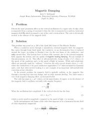
1. Wire with a Linearly Rising Current<br />
A neutral wire along the z-axis carries current I that varies with time t according to<br />
⎧<br />
⎪⎨ 0 (t ≤ 0),<br />
I(t)=<br />
⎪⎩ αt (t >0), α is a constant.<br />
Deduce the time-dependence of the electric and magnetic fields, E and B, observedat<br />
apoint(r, θ =0,z = 0) in a cylindrical coordinate system about the wire. Use your<br />
expressions to discuss the fields in the two limiting cases that ct ≫ r and ct = r + ɛ,<br />
where c is the speed of light and ɛ ≪ r.<br />
The related, but more intricate case of a solenoid with a linearly rising current is<br />
considered in http://puhep1.princeton.edu/~mcdonald/examples/solenoid.pdf<br />
(1)
<strong>Princeton</strong> <strong>University</strong> 2001 <strong>Ph501</strong> <strong>Set</strong> 8, <strong>Problem</strong> 2 2<br />
2. Harmonic Multipole Expansion<br />
A common alternative to the multipole expansion of electromagnetic radiation given in<br />
the Notes assumes from the beginning that the motion of the charges is oscillatory with<br />
angular frequency ω. However, we still use the essence of the Hertz method wherein<br />
the current density is related to the time derivative of a polarization: 1<br />
J = ṗ. (2)<br />
The radiation fields will be deduced from the retarded vector potential,<br />
A = 1 ∫ [J]<br />
c r<br />
dVol = 1 ∫ [ṗ]<br />
dVol, (3)<br />
c r<br />
which is a solution of the (Lorenz gauge) wave equation<br />
∇ 2 A − 1 ∂ 2 A<br />
c 2 ∂t = −4π J. (4)<br />
2 c<br />
Suppose that the Hertz polarization vector p has oscillatory time dependence,<br />
p(x,t)=p ω (x)e −iωt . (5)<br />
Using the expansion<br />
r = R − r ′ · ˆn + ... (6)<br />
of the distance r from source to observer,<br />
show that<br />
A = −iω ei(kR−ωt)<br />
cR<br />
∫<br />
( ( ) )<br />
1<br />
p ω (r ′ ) 1+r ′ · ˆn<br />
R − ik + ...<br />
dVol ′ , (7)<br />
where no assumption is made that R ≫ source size or that R ≫ λ =2π/k =2πc/ω.<br />
Consider now only the leading term in this expansion, which corresponds to electric<br />
dipole radiation. Introducing the total electric dipole moment,<br />
∫<br />
P ≡ p ω (r ′ ) dVol ′ , (8)<br />
1 Some consideration of the related topics of Hertz vectors and scalars is given in the Appendix of<br />
http://puhep1.princeton.edu/~mcdonald/examples/smallloop.pdf
<strong>Princeton</strong> <strong>University</strong> 2001 <strong>Ph501</strong> <strong>Set</strong> 8, <strong>Problem</strong> 2 3<br />
use<br />
B = ∇ × A and ∇ × B = 1 ∂E<br />
c ∂t<br />
to show that for an observer in vacuum the electric dipole radiation fields are<br />
B = k 2 ei(kR−ωt)<br />
R<br />
(9)<br />
(<br />
1+ i )<br />
ˆn × P, (10)<br />
kR<br />
{<br />
(<br />
E = k 2 ei(kR−ωt)<br />
1<br />
ˆn × (P × ˆn)+[3(ˆn · P)ˆn − P]<br />
R<br />
k 2 R − i )}<br />
. (11)<br />
2 kR<br />
Alternatively, deduce the electric field from both the scalar and vector potentials via<br />
E = −∇φ − 1 ∂A<br />
c ∂t , (12)<br />
in both the Lorenz and Coulomb gauges.<br />
For large R,<br />
B far ≈ k 2 ei(kR−ωt)<br />
ˆn × P,<br />
R<br />
E far ≈ B far × ˆn, (13)<br />
while for small R,<br />
B near ≈ ik<br />
R (ˆn × 3(ˆn · P)ˆn − P<br />
2 P)e−iωt , E near ≈ e −iωt , (14)<br />
R 3<br />
Thus, B near ≪ E near , and the electric field E near has the shape of the static dipole field<br />
of moment P, modulated at frequency ω.<br />
Calculate the Poynting vector of the fields of a Hertzian oscillating electric dipole (10)-<br />
(11) at all points in space. Show that the time-averaged Poynting vector has the same<br />
form in the near zone as it does in the far zone, which confirms that (classical) radiation<br />
exists both close to and far from the source.<br />
Extend your discussion to the case of an oscillating, point magnetic dipole by noting<br />
that if E(r,t)andB(r,t) are solutions to Maxwell’s equations in free space (i.e., where<br />
the charge density ρ and current density J are zero), then the dual fields<br />
are solutions also.<br />
E ′ (r,t)=−B(r,t), B ′ (r,t)=E(r,t), (15)
<strong>Princeton</strong> <strong>University</strong> 2001 <strong>Ph501</strong> <strong>Set</strong> 8, <strong>Problem</strong> 3 4<br />
3. Rotating Electric Dipole<br />
An electric dipole of moment p 0 lies in the x-y plane and rotates about the x axis with<br />
angular velocity ω.<br />
Calculate the radiation fields and the radiated power according to an observer at angle<br />
θ to the z axis in the x-z plane.<br />
Define ˆn towards the observer, so that ˆn · ẑ =cosθ, andletˆl = ŷ × ˆn.<br />
Show that<br />
B rad = p 0 k 2 ei(kr−ωt)<br />
(cos θ ŷ − i<br />
r<br />
ˆl),<br />
E rad = p 0 k 2 ei(kr−ωt)<br />
(cos θ<br />
r<br />
ˆl + i ŷ), (16)<br />
where r is the distance from the center of the dipole to the observer.<br />
Note that for an observer in the x-y plane (ˆn = ˆx), the radiation is linearly polarized,<br />
while for an observer along the z axis it is circularly polarized.<br />
Show that the (time-averaged) radiated power is given by<br />
d 〈P 〉<br />
dΩ<br />
= c<br />
8π p2 0 k4 (1 + cos 2 θ), 〈P 〉 = 2cp2 0k 4<br />
3<br />
= 2p2 0ω 4<br />
3c 3 . (17)<br />
This example gives another simple picture of how radiation fields are generated. The<br />
field lines emanating from the dipole become twisted into spirals as the dipole rotates.<br />
At large distances, the field lines are transverse...
<strong>Princeton</strong> <strong>University</strong> 2001 <strong>Ph501</strong> <strong>Set</strong> 8, <strong>Problem</strong> 4 5<br />
4. Magnetars<br />
The x-ray pulsar SGR1806-20 has recently been observed to have a period T of 7.5 s<br />
and a relatively large “spindown” rate ∣T<br />
˙<br />
∣ =8× 10 −11 . See, C. Kouveliotou et al., An<br />
X-ray pulsar with a superstrong magnetic field in the soft γ-ray repeater SGR1806-20,<br />
Nature 393, 235-237 (1998). 2<br />
Calculate the maximum magnetic field at the surface of this pulsar, assuming it to be<br />
a standard neutron star of mass 1.4M ⊙ =2.8 × 10 30 kg and radius 10 km, that the<br />
mass density is uniform, that the spindown is due to electromagnetic radiation, and<br />
that the angular velocity vector is perpendicular to the magnetic dipole moment of the<br />
pulsar.<br />
Compare the surface magnetic field strength to the so-called QED critical field strength<br />
m 2 c 3 /e¯h =4.4 × 10 13 gauss, at which electron-positron pair creation processes become<br />
highly probable.<br />
2 http://puhep1.princeton.edu/~mcdonald/examples/EM/kouveliotou_nature_393_235_98.pdf
<strong>Princeton</strong> <strong>University</strong> 2001 <strong>Ph501</strong> <strong>Set</strong> 8, <strong>Problem</strong> 5 6<br />
5. Radiation of Angular Momentum<br />
Recall that we identified a field momentum density,<br />
and angular momentum density<br />
P field = S c 2 = U c ˆk, (18)<br />
L field = r × P field . (19)<br />
Show that for oscillatory sources, the time-average angular momentum radiated in unit<br />
solid angle per second is (the real part of)<br />
d 〈L〉<br />
dt dΩ = 1<br />
8π r3 [E(ˆn · B ⋆ ) − B ⋆ (ˆn · E)]. (20)<br />
Thus, the radiated angular momentum is zero for purely transverse fields.<br />
In prob. 2, eq. (11) we found that for electric dipole radiation there is a term in E with<br />
E · ˆn ∝ 1/r 2 . Show that for radiation by an oscillating electric dipole p,<br />
d 〈L〉<br />
dt dΩ = ik3<br />
4π (ˆn · p)(ˆn × p⋆ ). (21)<br />
Ifthedipolemomentp is real, eq. (21) tells us that no angular momentum is radiated.<br />
However, when p is real, the radiation is linearly polarized and we expect it to carry<br />
no angular momentum.<br />
Rather, we need circular (or elliptical) polarization to have radiated angular momentum.<br />
The radiation fields (16) of prob. 2 are elliptically polarized. Show that in this case<br />
the radiated angular momentum distribution is<br />
d 〈L〉<br />
dt dΩ = − k3<br />
4π p2 0 sin θˆl,<br />
and<br />
d 〈L〉<br />
dt<br />
= 〈P 〉 ẑ. (22)<br />
ω<br />
[These relations carry over into the quantum realm where a single (left-hand) circularly<br />
polarized photon has U =¯hω, p =¯hk, andL =¯h.<br />
For a another view of waves that carry angular momentum, see<br />
http://puhep1.princeton.edu/~mcdonald/examples/oblate_wave.pdf
<strong>Princeton</strong> <strong>University</strong> 2001 <strong>Ph501</strong> <strong>Set</strong> 8, <strong>Problem</strong> 6 7<br />
6. Oscillating Electric Quadrupole<br />
An oscillating linear quadrupole consists of charge 2e at the origin, and two charges<br />
−e each at z = ±a cos ωt.<br />
Show that for an observer in the x-z plane at distance r from the origin,<br />
E rad = −4k 3 a 2 sin(2kr − 2ωt)<br />
e sin θ cos θ<br />
r<br />
ˆl, (23)<br />
where ˆl = ŷ × ˆn. This radiation is linearly polarized.<br />
Show also that the time-averaged total power is<br />
〈P 〉 = 16<br />
15 ck6 a 4 e 2 . (24)
<strong>Princeton</strong> <strong>University</strong> 2001 <strong>Ph501</strong> <strong>Set</strong> 8, <strong>Problem</strong> 7 8<br />
7. A single charge e rotates in a circle of radius a with angular velocity ω. The circle is<br />
centered in the x-y plane.<br />
The time-varying electric dipole moment of this charge distribution with respect to the<br />
origin has magnitude p = ae, so from Larmor’s formula (prob. 2) we know that the<br />
(time-averaged) power in electric dipole radiation is<br />
〈P E1 〉 = 2a2 e 2 ω 4<br />
3c 3 . (25)<br />
This charge distribution also has a magnetic dipole moment and an electric quadrupole<br />
moment (plus higher moments as well!). Calculate the total radiation fields due to the<br />
E1, M1 and E2 moments, as well as the angular distribution of the radiated power and<br />
the total radiated power from these three moments. In this pedagogic problem you<br />
may ignore the interference between the various moments.<br />
Show, for example, that the part of the radiation due only to the electric quadrupole<br />
moment obeys<br />
d 〈P E2 〉<br />
dΩ = a4 e 2 ω 6<br />
2πc 5 (1 − cos4 θ), 〈P E2 〉 = 8a4 e 2 ω 6<br />
5c 5 . (26)<br />
Thus,<br />
〈P E2 〉<br />
〈P E1 〉 = 12a2 ω 2<br />
5c 2<br />
where v = aω is the speed of the charge.<br />
∝ v2<br />
c 2 , (27)
<strong>Princeton</strong> <strong>University</strong> 2001 <strong>Ph501</strong> <strong>Set</strong> 8, <strong>Problem</strong> 8 9<br />
8. Radiation by a Classical Atom<br />
a) Consider a classical atom consisting of charge +e fixed at the origin, and charge −e<br />
in a circular orbit of radius a. As in prob. 5, this atom emits electric dipole radiation<br />
⇒ loss of energy ⇒ the electron falls into the nucleus!<br />
Calculate the time to fall to the origin supposing the electron’s motion is nearly circular<br />
at all times (i.e., it spirals into the origin with only a small change in radius per turn).<br />
You may ignore relativistic corrections. Show that<br />
t fall =<br />
a3<br />
4r 2 0c , (28)<br />
where r 0 = e 2 /mc 2 is the classical electron radius. Evaluate t fall for a =5× 10 −9 cm<br />
= the Bohr radius.<br />
b) The energy loss of part a) can be written as<br />
dU<br />
dt = P dipole ∝ e2 aω 4<br />
c<br />
= e2<br />
a<br />
( aω<br />
c<br />
or<br />
dipole energy loss per revolution<br />
energy<br />
For quadrupole radiation, prob. 5 shows that<br />
) 3 ( ) v 3<br />
ω ∝ U ω ∝ U ( ) v 3<br />
, (29)<br />
c T c<br />
( ) v 3<br />
∝ . (30)<br />
c<br />
quadrupole energy loss per revolution<br />
energy<br />
( ) v 5<br />
∝ . (31)<br />
c<br />
Consider the Earth-Sun system. The motion of the Earth around the Sun causes a<br />
quadrupole moment, so gravitational radiation is emitted (although, of course, there<br />
is no dipole gravitational radiation since the dipole moment of any system of masses<br />
about its center of mass is zero). Estimate the time for the Earth to fall into the Sun<br />
due to gravitational radiation loss.<br />
What is the analog of the factor ea 2 that appears in the electrical quadrupole moment<br />
(prob. 5) for masses m 1 and m 2 that are in circular motion about each other, separated<br />
by distance a?<br />
Also note that in Gaussian units the electrical coupling constant k in the force law<br />
F = ke 1 e 2 /r 2 has been set to 1, but for gravity k = G, Newton’s constant.<br />
The general relativity expression for quadrupole radiation in the present example is<br />
P G2 = 32 5<br />
G<br />
c 5 m 2 1 m2 2<br />
(m 1 + m 2 ) 2 a4 ω 6 (32)<br />
[Phys. Rev. 131, 435 (1963)]. The extra factor of 4 compared to E2 radiation arises<br />
because the source term in the gravitational wave equation has a factor of 16π, rather<br />
than 4π as for E&M.
<strong>Princeton</strong> <strong>University</strong> 2001 <strong>Ph501</strong> <strong>Set</strong> 8, <strong>Problem</strong> 9 10<br />
9. Why Doesn’t a Steady Current Loop Radiate?<br />
A steady current in a circular loop presumably involves a large number of electrons in<br />
uniform circular motion. Each electron undergoes accelerated motion, and according<br />
to prob. 5 emits radiation. Yet, the current density J is independent of time in the<br />
limit of a continuous current distribution, and therefore does not radiate. How can we<br />
reconcile these two views?<br />
The answer must be that the radiation is canceled by destructive interference between<br />
the radiation fields of the large number N of electrons that make up the steady current.<br />
Prob. 5 showed that a single electron in uniform circular motion emits electric dipole radiation,<br />
whose power is proportional to (v/c) 4 . But the electric dipole moment vanishes<br />
for two electrons in uniform circular motion at opposite ends of a common diameter;<br />
quadrupole radiation is the highest multipole in this case, with power proportional to<br />
(v/c) 6 . It is suggestive that in case of 3 electrons 120 ◦ apart in uniform circular motion<br />
the (time-dependent) quadrupole moment vanishes, and the highest multipole radiation<br />
is octupole. For N electrons evenly spaced around a ring, the highest multipole<br />
that radiates in the Nth, and the power of this radiation is proportional to (v/c) 2N+2 .<br />
Then, for steady motion with v/c ≪ 1, the radiated power of a ring of N electrons is<br />
very small.<br />
Verify this argument with a detailed calculation.<br />
Since we do not have on record a time-dependent multipole expansion to arbitrary<br />
order, return to the basic expression for the vector potential of the radiation fields,<br />
A(r,t)= 1 c<br />
∫ [J]<br />
r dVol′ ≈ 1 ∫<br />
cR<br />
[J] dVol ′ = 1 ∫<br />
cR<br />
J(r ′ ,t ′ = t − r/c) dVol ′ , (33)<br />
where R is the (large) distance from the observer to the center of the ring of radius<br />
a. For uniform circular motion of N electrons with angular frequency ω, the current<br />
density J is a periodic function with period T =2π/ω, so a Fourier analysis can be<br />
made where<br />
∞∑<br />
J(r ′ ,t ′ )= J m (r ′ )e −imωt′ , (34)<br />
m=−∞<br />
with<br />
J m (r ′ )= 1 ∫ T<br />
J(r ′ ,t ′ )e imωt′ dt ′ .<br />
T 0<br />
(35)<br />
Then,<br />
A(r,t)= ∑ A m (r)e −imωt ,<br />
m<br />
(36)<br />
etc.<br />
The radiated power follows from the Poynting vector,<br />
dP<br />
dΩ = c<br />
4π R2 |B| 2 = c<br />
4π R2 |∇ × A| 2 . (37)<br />
However, as discussed on p. 181 of the Notes, one must be careful in going from a<br />
Fourier analysis of an amplitude, such as B, to a Fourier analysis of an intensity that
<strong>Princeton</strong> <strong>University</strong> 2001 <strong>Ph501</strong> <strong>Set</strong> 8, <strong>Problem</strong> 9 11<br />
depends on the square of the amplitude. Transcribing the argument there to the present<br />
case, a Fourier analysis of the average power radiated during one period T can be given<br />
as<br />
d 〈P 〉<br />
dΩ<br />
∫ T<br />
∫ T<br />
= 1 dP cR2<br />
dt = |B| 2 dt = cR2<br />
T 0 dΩ 4πT 0<br />
4πT 0<br />
= cR2 ∑<br />
∫<br />
1 T<br />
B m B ⋆ e −imωt dt = cR2 ∞∑<br />
4π m T 0<br />
4π<br />
= cR2 ∞∑<br />
∞∑<br />
|B m | 2 ≡<br />
2π<br />
m=0<br />
m=0<br />
∫ T<br />
B ⋆ ∑ m<br />
m=−∞<br />
B m B ⋆ m<br />
B m e −imωt dt<br />
dP m<br />
dΩ . (38)<br />
That is, the Fourier components of the time-averaged radiated power can be written<br />
dP m<br />
dΩ = cR2<br />
2π |B m| 2 = cR2<br />
2π |∇ × A m| 2 = cR2<br />
2π |imkˆn × A m| 2 , (39)<br />
where k = ω/c and ˆn points from the center of the ring to the observer.<br />
Evaluate the Fourier components of the vector potential and of the radiated power<br />
first for a single electron, with geometry as in prob. 5, and then for N electrons evenly<br />
spaced around the ring. It will come as no surprise that a 3-dimensional problem with<br />
charges distributed on a ring leads to Bessel functions, and we must be aware of the<br />
integral representation<br />
∫<br />
J m (z) = im 2π<br />
e imφ−iz cos φ dφ. (40)<br />
2π 0<br />
Use the asymptotic expansion for large index and small argument,<br />
J m (mx) ≈ (ex/2)m √<br />
2πm<br />
(m ≫ 1, x≪ 1), (41)<br />
to verify the suppression of the radiation for large N.<br />
This problem was first posed (and solved via series expansions without explicit mention<br />
of Bessel functions) by J.J. Thomson, Phil. Mag. 45, 673 (1903). 3 He knew that atoms<br />
(in what we now call their ground state) don’t radiate, and used this calculation to<br />
support his model that the electric charge in an atom must be smoothly distributed.<br />
This was a classical precursor to the view of a continuous probability distribution for<br />
the electron’s position in an atom.<br />
Thomson’s work was followed shortly by an extensive treatise by G.A. Schott, Electromagnetic<br />
Radiation (Cambridge U.P., 1912), that included analyses in term of Bessel<br />
functions correct for any value of v/c.<br />
These pioneering works were largely forgotten during the following era of nonrelativistic<br />
quantum mechanics, and were reinvented around 1945 when interest emerged in<br />
relativistic particle accelerators. See Arzimovitch and Pomeranchuk, 4 and Schwinger. 5<br />
3 http://puhep1.princeton.edu/~mcdonald/examples/EM/thomson_pm_45_673_03.pdf<br />
4 http://puhep1.princeton.edu/~mcdonald/examples/EM/arzimovitch_jpussr_9_267_45.pdf<br />
5 http://puhep1.princeton.edu/~mcdonald/accel/schwinger.pdf
<strong>Princeton</strong> <strong>University</strong> 2001 <strong>Ph501</strong> <strong>Set</strong> 8, <strong>Problem</strong> 10 12<br />
10. Spherical Cavity Radiation<br />
Thus far we have only considered waves arising from the retarded potentials, and have<br />
ignored solutions via the advanced potentials. “Advanced” spherical waves converge<br />
on the source rather than propagate away – so we usually ignore them.<br />
Inside a cavity, an outward going wave can bounce off the walls and become an inward<br />
going wave. Thus, a general description of cavity radiation should include both kinds<br />
of waves.<br />
Reconsider your derivation in Prob. 1, this time emphasizing the advanced waves, for<br />
which t ′ = t + r/c is the “advanced” time. It suffices to consider only the fields due to<br />
oscillation of an electric dipole moment.<br />
If one superimposes outgoing waves due to oscillating dipole p = p 0 e −iωt at the origin<br />
with incoming waves associated with dipole −p, then we can have standing waves –<br />
and zero total dipole moment.<br />
Suppose all this occurs inside a spherical cavity with perfectly conducting walls at<br />
radius a. Show that the condition for standing waves associated with the virtual<br />
electric dipole is<br />
cot ka = 1<br />
ka − ka ⇒ ω min =2.74 c a , (42)<br />
where k = ω/c. [A quick estimate would be λ max =2a ⇒ ω min = πc/a.]<br />
By a simple transformation, use your result to find the condition for standing magnetic<br />
dipoles waves inside a spherical cavity:<br />
tan ka = ka ⇒ ω min =4.49 c a . (43)
<strong>Princeton</strong> <strong>University</strong> 2001 <strong>Ph501</strong> <strong>Set</strong> 8, <strong>Problem</strong> 11 13<br />
11. Maximum Energy of a Betatron<br />
A betatron is a circular device of radius R designed to accelerate electrons (charge e,<br />
mass m) via a changing magnetic flux ˙Φ =πR 2 Ḃ ave through the circle.<br />
Deduce the relation between the magnetic field B at radius R and the magnetic field<br />
B ave averaged over the area of the circle needed for a betatron to function. Also deduce<br />
the maximum energy E to which an electron could be accelerated by a betatron in terms<br />
of B, Ḃ ave and R.<br />
Hints: The electrons in this problem are relativistic, so it is useful to introduce the<br />
factor γ = E/mc 2 where c is the speed of light. Recall that Newton’s second law has<br />
the same form for nonrelativistic and relativistic electrons except that in the latter case<br />
the effective mass is γm. Recall also that for circular motion the rest frame acceleration<br />
is γ 2 times that in the lab frame.
<strong>Princeton</strong> <strong>University</strong> 2001 <strong>Ph501</strong> <strong>Set</strong> 8, <strong>Problem</strong> 12 14<br />
12. a) An oscillating electric dipole of angular frequency ω is located at distance d ≪ λ<br />
away from a perfectly conducting plane. The dipole is oriented parallel to the plane,<br />
as shown below.<br />
Show that the power radiated in the direction (θ, φ) is<br />
dP<br />
dΩ =4A sin2 θ sin 2 Δ, (44)<br />
where<br />
Δ= 2πλ sin θ cos φ, (45)<br />
d<br />
and the power radiated by the dipole alone is<br />
dP<br />
dΩ = A sin2 θ. (46)<br />
Sketch the shape of the radiation pattern for d = λ/2 andd = λ/4.<br />
b) Suppose instead that the dipole was oriented perpendicular to the conducting plane.<br />
Show that the radiated power in this case is<br />
dP<br />
dΩ =4A sin2 θ ′ cos 2 Δ, (47)<br />
where<br />
Δ= 2πλ<br />
d cos θ′ . (48)<br />
In parts a) and b), the polar angles θ and θ ′ are measured with respect to the axes of<br />
the dipoles.<br />
c) Repeat parts a) and b) for a magnetic dipole oscillator in the two orientations.
<strong>Princeton</strong> <strong>University</strong> 2001 <strong>Ph501</strong> <strong>Set</strong> 8, <strong>Problem</strong> 13 15<br />
13. In an array of antennas, their relative phases can be adjusted as well as their relative<br />
spacing, which leads to additional freedom to shape the radiation pattern.<br />
Consider two short, center-fed linear antennas of length L ≪ λ, peak current I 0 and<br />
frequency ω, as discussed on p. 191 of the Notes. The axes of the antennas are collinear,<br />
their centers are λ/4 apart, and the currents have a 90 ◦ phase difference.<br />
Show that the angular distribution of the radiated power is<br />
dU<br />
dtdΩ =<br />
[ ( )]<br />
ω2<br />
π<br />
16πc I 0L 2 2 sin 2 θ 1+sin<br />
3 2 cos θ . (49)<br />
Unlike the radiation patterns of previous examples, this is not symmetric about the<br />
plane z = 0. Therefore, this antenna array emits nonzero momentum P rad . As a<br />
consequence, there is a net reaction force F = −dP rad /dt. Show that<br />
F = − 1 c<br />
dU<br />
dt<br />
( )<br />
1 − π2<br />
ẑ. (50)<br />
12<br />
A variant on this problem is at<br />
http://puhep1.princeton.edu/~mcdonald/examples/endfire.pdf
<strong>Princeton</strong> <strong>University</strong> 2001 <strong>Ph501</strong> <strong>Set</strong> 8, <strong>Problem</strong> 14 16<br />
14. a) Consider a full-wave “end-fire” antenna whose current distribution (along the z axis)<br />
is<br />
I(z) =I 0 sin 2πz<br />
L e−iωt , (−L/2
<strong>Princeton</strong> <strong>University</strong> 2001 <strong>Ph501</strong> <strong>Set</strong> 8, <strong>Problem</strong> 15 17<br />
15. Scattering Off a Conducting Sphere<br />
Calculate the scattering cross section for plane electromagnetic waves of angular frequency<br />
ω incident on a perfectly conducting sphere of radius a when the wavelength<br />
obeys λ ≫ a (ka ≪ 1).<br />
Note that both electric and magnetic dipole moments are induced. Inside the sphere,<br />
B total must vanish. Surface currents are generated such that B induced = −B incident ,and<br />
because of the long wavelength, these fields are essentially uniform over the sphere.<br />
(c.f. <strong>Set</strong> 4, Prob. 8a).<br />
Show that<br />
[<br />
E scat = a 3 k 2 ei(kr−ωt)<br />
(E 0 × ˆn) × ˆn − 1 ]<br />
r<br />
2 (B 0 × ˆn , (57)<br />
where ˆn is along the vector r that points from the center of the sphere to the distant<br />
observer.<br />
Suppose that the incident wave propagates in the +z direction, and the electric field<br />
is linearly polarized along direction ˆl, soE 0 = E 0ˆl and ˆl · ẑ = 0. Show that in this case<br />
the scattering cross section can be written,<br />
⎡(<br />
dσ<br />
dΩ = a6 k 4 ⎣ 1 − ˆn · ẑ ) ⎤<br />
2<br />
− 3 2 4 (ˆl · ˆn) 2 ⎦ . (58)<br />
Consider an observer in the x-z plane to distinguish between the cases of electric<br />
polarization parallel and perpendicular to the scattering plane to show that<br />
dσ ‖<br />
dΩ = a6 k 4 ( 1<br />
2 − cos θ ) 2<br />
,<br />
(<br />
dσ ⊥<br />
dΩ = a6 k 4 1 − cos θ ) 2<br />
. (59)<br />
2<br />
Then, for an unpolarized incident wave, show<br />
[ ]<br />
dσ 5<br />
dΩ = a6 k 4 8 (1 + cos2 θ) − cos θ , (60)<br />
and<br />
∫ dσ<br />
σ =<br />
dΩ dΩ=10π 3 a6 k 4 . (61)<br />
Sketch the angular distribution (60). Note that<br />
dσ(180 ◦ /<br />
) dσ(0 ◦ )<br />
=9, (62)<br />
dΩ dΩ<br />
so the sphere reflects much more backwards than it radiates forwards.<br />
Is there any angle θ for which the scattered radiation is linearly polarized for unpolarized<br />
incident waves?
<strong>Princeton</strong> <strong>University</strong> 2001 <strong>Ph501</strong> <strong>Set</strong> 8, <strong>Problem</strong> 16 18<br />
16. Exotic radiation effects of charges that move at (essentially) constant velocity but<br />
cross boundaries between various media can be deduced from the radiation spectrum<br />
equation (14.70) from the textbook of Jackson (p. 182 of the Notes):<br />
dU<br />
dωdΩ =<br />
[∫<br />
ω2<br />
4π 2 c 3<br />
dt d 3 r ˆn × J(r,t)e iω(t−(ˆn·r)/c) ] 2<br />
, (63)<br />
where dU is the radiated energy in angular frequency interval dω emitting into solid<br />
angle dΩ, J is the source current density, and ˆn is a unit vector towards the observer.<br />
Consider the example of the sweeping electron beam in an (analog) oscilloscope. In the<br />
fastest of such devices (such as the Tektronix model 7104) the speed of the beam spot<br />
across the face of an oscilloscope can exceed the velocity of light, although of course<br />
the velocity of the electrons does not. Associated with this possibility there should be<br />
akindofČerenkov radiation, as if the oscilloscope trace were due to a charge moving<br />
with superluminal velocity.<br />
As a simple model, suppose a line of charge moves in the −y direction with velocity<br />
u ≪ c, wherec is the speed of light, but has a slope such that the intercept with the<br />
x axis moves with velocity v>c, as shown in the figure below. If the region yc.Asthe<br />
charge disappears into the conductor at y
<strong>Princeton</strong> <strong>University</strong> 2001 <strong>Ph501</strong> <strong>Set</strong> 8, Solution 1 19<br />
Solutions<br />
1. The suggested approach is to calculate the retarded potentials and then take derivatives<br />
to find the fields. The retarded scalar and vector potentials φ and A are given by<br />
∫ ρ(x ′ ,t− R/c)<br />
φ(x,t)=<br />
d 3 x ′ , and A(x,t)= 1 ∫ J(x ′ ,t− R/c)<br />
d 3 x ′ , (64)<br />
R<br />
c R<br />
where ρ and J are the charge and current densities, respectively, and R = |x − x ′ |.<br />
In the present case, we assume the wire remains neutral when the current flows (compare<br />
Prob. 3, <strong>Set</strong> 4). Then the scalar potential vanishes. For the vector potential, we<br />
see that only the component A z will be nonzero. Also, J d 3 x ′ can be rewritten as Idzfor<br />
current in a wire along the z-axis. Foranobserverat(r, 0, 0) and a current element at<br />
(0, 0,z), we have R = √ r 2 + z 2 . Further, the condition that I is nonzero only for time<br />
t>0 implies that it contributes to the fields only for z such that (ct) 2 >R 2 = r 2 + z 2 .<br />
That is, we need to evaluate the integral only for<br />
√<br />
|z|
<strong>Princeton</strong> <strong>University</strong> 2001 <strong>Ph501</strong> <strong>Set</strong> 8, Solution 1 20<br />
so<br />
B φ ≈ 2α<br />
√<br />
2ɛ<br />
c 2 r , and E z ≈− 2α<br />
c ln r + ɛ + √ 2rɛ<br />
2 r<br />
≈− 2α<br />
c 2 √<br />
2ɛ<br />
r = −B φ. (71)<br />
In this regime, the fields have the character of radiation, with E and B of equal<br />
magnitude, mutually orthogonal, and both orthogonal to the line of sight to the closest<br />
point on the wire. (Because of the cylindrical geometry the radiation fields do not have<br />
1/r dependence – which holds instead for static fields.)<br />
In sum, the fields build up from zero only after time ct = r. The initial fields propagate<br />
outwards at the speed of light and have the character of cylindrical waves. But at a<br />
fixed r, the electric field dies out with time, and the magnetic field approaches the<br />
instantaneous magnetostatic field due to the current in the wire.<br />
Of possible amusement is a direct calculation of the vector potential for the case of a<br />
constant current I 0 .<br />
First, from Ampere’s law we know that B φ =2I 0 /cr = −∂A z /∂r, sowehavethat<br />
A z = − 2I 0<br />
ln r + const. (72)<br />
c<br />
Whereas, if we use the integral form for the vector potential we have<br />
A z (r, 0, 0) = 1 ∫ ∞ I 0 dz<br />
√<br />
c −∞ r2 + z = 2I ∫ ∞<br />
0 dz<br />
√ 2 c 0 r2 + z 2<br />
= − 2I 0<br />
c<br />
ln r + lim<br />
z→∞ ln(z + √ z 2 + r 2 ). (73)<br />
Only by ignoring the last term, which does not depend on r for a long wire, do we<br />
recover the “elementary” result.
<strong>Princeton</strong> <strong>University</strong> 2001 <strong>Ph501</strong> <strong>Set</strong> 8, Solution 2 21<br />
2. The expansion<br />
r = R − r ′ · ˆn + ... (74)<br />
implies that the retarded time derivative of the polarization vector is<br />
[ṗ] = ṗ(r ′ ,t ′ = t − r/c) ≈−iωp ω (r ′ )e −iω(t−R/c+r′·ˆn/c) = −iωe i(kR−ωt) p ω (r ′ )e −ikr′·ˆn<br />
≈ −iωe i(kR−ωt) p ω (r ′ )(1 − ikr ′ · ˆn), (75)<br />
where k = ω/c. Likewise,<br />
1<br />
r ≈ 1 ( )<br />
1+ r′ · ˆn<br />
. (76)<br />
R R<br />
Then, the retarded vector potential can be written (in the Lorenz gauge)<br />
A (L) = 1 c<br />
∫ [ṗ]<br />
r<br />
dVol′ ≈−iω ei(kR−ωt)<br />
cR<br />
∫<br />
[ ( ) ]<br />
1<br />
p ω (r ′ ) 1+r ′ · ˆn<br />
R − ik + ...<br />
dVol ′ , (77)<br />
Theelectricdipole(E1) approximation is to keep only the first term of eq. (77),<br />
∫<br />
A (L)<br />
E1 = −iω ei(kR−ωt)<br />
cR<br />
p ω (r ′ ) dVol ′ ≡−ik ei(kR−ωt)<br />
P (Lorenz gauge). (78)<br />
R<br />
We obtain the magnetic field by taking the curl of eq. (78). The curl operation with<br />
respect to the observer acts only on the distance R. In particular,<br />
∇R = R R<br />
= ˆn. (79)<br />
Hence,<br />
B E1 = ∇ × A (L)<br />
E1 = −ik∇ei(kR−ωt)<br />
R<br />
= k 2 ei(kR−ωt)<br />
R<br />
× P = −ik ei(kR−ωt)<br />
ikˆn − ˆn × P<br />
R<br />
R<br />
(<br />
1+ i )<br />
ˆn × P. (80)<br />
kR<br />
The 4th Maxwell equation in vacuum tells us that<br />
∇ × B E1 = 1 ∂E E1<br />
= −ikE E1 .<br />
c ∂t<br />
(81)<br />
Hence,<br />
E E1 = i [ ( ik<br />
k ∇ × B E1 = ∇ × e i(kR−ωt) R − 1 ) ]<br />
R × P<br />
2 R 3<br />
( ik<br />
= ∇e i(kR−ωt) R − 1 )<br />
( ik<br />
× (R × P)+e i(kR−ωt) 2 R 3 R − 1 )<br />
∇ × (R × P)<br />
2 R 3<br />
[ (<br />
= e i(kR−ωt) − k2 ik<br />
R − 3 R − 1 )]<br />
( ik<br />
ˆn × (ˆn × P) − 2Pe i(kR−ωt) 2 R 3 R − 1 )<br />
2 R 3<br />
(<br />
= k 2 ei(kR−ωt)<br />
ik<br />
ˆn × (P × ˆn)+e i(kR−ωt)<br />
R<br />
R − 1 )<br />
[P − 3(P · ˆn)ˆn]. (82)<br />
2 R 3<br />
(<br />
)
<strong>Princeton</strong> <strong>University</strong> 2001 <strong>Ph501</strong> <strong>Set</strong> 8, Solution 2 22<br />
We could also deduce the electric field from the general relation<br />
E = −∇V − 1 c<br />
∂A<br />
∂t<br />
= −∇V + ikA. (83)<br />
For this, we need to know the scalar potential V (L) , which we can deduce from the<br />
Lorenz gauge condition:<br />
∇ · A (L) + 1 c<br />
For an oscillatory source this becomes<br />
∂V (L)<br />
In the electric dipole approximation (78) this yields 6<br />
V (L)<br />
E1<br />
= e i(kR−ωt) ( 1<br />
R 2 − ik R<br />
∂t<br />
=0. (84)<br />
V (L) = − i k ∇ · A(L) . (85)<br />
For small R the scalar potential is that of a time-varying dipole,<br />
)<br />
(P · ˆn) (Lorenz gauge). (86)<br />
The electric field is given by<br />
V (L)<br />
E1,near ≈ P · ˆn<br />
R 2 e−iωt . (87)<br />
E E1 = −∇V (L)<br />
E1<br />
+ ikA (L)<br />
E1<br />
( ik<br />
= (P · R)∇e i(kR−ωt) R − 1 )<br />
( ik<br />
+ e i(kR−ωt) 2 R 3 R − 1 )<br />
2 R 3<br />
[<br />
= e i(kR−ωt)<br />
− k2<br />
R − 3 ( ik<br />
R 2 − 1 R 3 )]<br />
(P · ˆn)ˆn + e i(kR−ωt) ( ik<br />
R 2 − 1 R 3 )<br />
P<br />
∇(P · R)+k 2 ei(kR−ωt)<br />
R<br />
P<br />
+k 2 ei(kR−ωt)<br />
R<br />
P<br />
(<br />
= k 2 ei(kR−ωt)<br />
ik<br />
ˆn × (P × ˆn)+e i(kR−ωt)<br />
R<br />
R − 1 )<br />
[P − 3(P · ˆn)ˆn], (88)<br />
2 R 3<br />
as before. The angular distribution in the far field (for which the radial dependence is<br />
1/R) isˆn×(P× ˆn) =P−(P· ˆn)ˆn. The isotropic term P is due to the vector potential,<br />
while the variable term −(P · ˆn)ˆn is due to the scalar potential and is purely radial.<br />
Spherical waves associated with a scalar potential must be radial (longitudinal), but<br />
the transverse character of electromagnetic waves in the far field does not imply the<br />
absence of a contribution of the scalar potential; the latter is needed (in the Lorenz<br />
gauge) to cancel to radial component of the waves from the vector potential.<br />
6 Equation (86) is not simply the electrostatic dipole potential times a spherical wave because the retarded<br />
positions at time t of the two charges of a point dipole correspond to two different retarded times t ′ .<br />
For a calculation of the retarded scalar potential via V (L) = ∫ [ρ]/r, see sec. 11.1.2 of Introduction to<br />
Vol<br />
<strong>Electrodynamics</strong> by D.J. Griffiths.
<strong>Princeton</strong> <strong>University</strong> 2001 <strong>Ph501</strong> <strong>Set</strong> 8, Solution 2 23<br />
We could also work in the Coulomb gauge, meaning that we set ∇ · A (C) = 0. Recall<br />
(Lecture 15, p. 174) that the “wave” equations for the potentials in the Coulomb gauge<br />
are<br />
∇ 2 V (C) = −4πρ, (89)<br />
∇ 2 A (C) − 1 ∂ 2 A (C)<br />
= − 4π c 2 ∂t 2 c J + 1 ∂∇V (C)<br />
. (90)<br />
c ∂t<br />
Equation (89) is the familiar Poisson equation of electrostatics, so the scalar potential<br />
is just the “instantaneous” electric-dipole potential,<br />
V (C)<br />
E1<br />
= P · ˆn<br />
R 2 e−iωt (Coulomb gauge). (91)<br />
One way to deduce the Coulomb-gauge vector potential is via eq. (83),<br />
A (C)<br />
E1 = − i k E E1 − i (C)<br />
∇V E1<br />
k<br />
= −ik ei(kR−ωt)<br />
ˆn × (P × ˆn)+<br />
R<br />
≡<br />
A (C)<br />
far<br />
[ e<br />
i(kR−ωt)<br />
+ i(ei(kR−ωt) − e −iωt ]<br />
)<br />
[P − 3(P · ˆn)ˆn]<br />
R 2 kR 3<br />
+ A (C)<br />
near (Coulomb gauge). (92)<br />
We learn that the far-zone, Coulomb gauge vector potential (i.e., the part of the vector<br />
potential that varies as 1/R) is purely transverse, and can be written as<br />
A (C)<br />
far<br />
= −ik ei(kR−ωt)<br />
ˆn × (P × ˆn) (Coulomb gauge). (93)<br />
R<br />
Because the radiation part of the Coulomb-gauge vector potential is transverse, the<br />
Coulomb gauge is sometimes called the “transverse” gauge.<br />
The Coulomb-gauge scalar potential is negligible in the far zone, and we can say that<br />
the radiation fields are entirely due to the far-zone, Coulomb-gauge vector potential.<br />
That is,<br />
E far = ikA (C)<br />
far<br />
B far = ∇ × A (C)<br />
far<br />
= k 2 ei(kR−ωt)<br />
ˆn × (P × ˆn), (94)<br />
R<br />
= ik × A (C)<br />
far<br />
= k 2 ei(kR−ωt)<br />
ˆn × P. (95)<br />
R<br />
It is possible to choose gauges for the electromagnetic potentials such that some of<br />
their components appear to propagate at any velocity v, as discussed by J.D. Jackson,<br />
Am. J. Phys. 70, 917 (2002) and by K.-H. Yang, Am. J. Phys. 73, 742 (2005). 7 The<br />
7 http://puhep1.princeton.edu/~mcdonald/examples/EM/jackson_ajp_70_917_02.pdf<br />
http://puhep1.princeton.edu/~mcdonald/examples/EM/yang_ajp_73_742_05.pdf
<strong>Princeton</strong> <strong>University</strong> 2001 <strong>Ph501</strong> <strong>Set</strong> 8, Solution 2 24<br />
potentials A (v) and V (v) in the so-called velocity gauge with the parameter v obey the<br />
gauge condition<br />
∇ · A (v) + c ∂V (v)<br />
=0. (96)<br />
v 2 ∂t<br />
The scalar potential V (v) is obtained by replacing the speed of light c in the Lorenzgauge<br />
scalar potential by v. Equivalently, we replace the wave number k = ω/c by<br />
k ′ = ω/v. Thus, from eq. (86) we find<br />
V (v)<br />
E1<br />
= −ei(k′ R−ωt)<br />
(<br />
ik<br />
′<br />
R 2 − 1 R 3 )<br />
(P · R) (velocity gauge). (97)<br />
Then, as in eq. (88) we obtain<br />
− ∇V (v)<br />
E1 = e i(k′ R−ωt)<br />
[− k′ 2 (<br />
ik<br />
′<br />
R − 3 R − 1 )]<br />
(<br />
ik<br />
(P · ˆn)ˆn + e i(kR−ωt) ′<br />
2 R 3 R − 1 )<br />
P<br />
2 R 3<br />
(<br />
= −k ′ 2 e i(k′ R−ωt)<br />
(P · ˆn)ˆn + e i(k′ R−ωt) ik<br />
′<br />
R<br />
R − 1 )<br />
[P − 3(P · ˆn)ˆn]. (98)<br />
2 R 3<br />
The vector potential in the v-gauge can be obtained from eq. (83) as<br />
A (v)<br />
E1 = − i k E E1 − i (v)<br />
∇V E1<br />
k<br />
(<br />
= −ik ei(kR−ωt)<br />
1<br />
ˆn × (P × ˆn)+e i(kR−ωt)<br />
R<br />
R + 2<br />
−i k′ 2<br />
(<br />
e i(k′ R−ωt)<br />
(P · ˆn)ˆn − e i(k′ R−ωt) k<br />
′<br />
k R<br />
kR + 2<br />
i )<br />
[P − 3(P · ˆn)ˆn]<br />
kR 3<br />
i )<br />
[P − 3(P · ˆn)ˆn]. (99)<br />
kR 3<br />
This vector potential includes terms that propagate with velocity v both in the near<br />
and far zones. When v = c, thenk ′ = k and the velocity-gauge vector potential (99)<br />
reduces to the Lorenz-gauge potential (78); and when v →∞,thenk ′ =0and the<br />
velocity-gauge vector potential reduces to the Coulomb-gauge potential (92). 8<br />
Turning to the question of energy flow, we calculate the Poynting vector<br />
S = c E × B, (100)<br />
4π<br />
where we use the real parts of the fields (80) and (82),<br />
E = k 2 P ˆn×( ˆP× ˆn)<br />
[ ]<br />
cos(kR − ωt)<br />
+P [3ˆP· ˆn)ˆn−<br />
R<br />
ˆP] cos(kR − ωt) k sin(kR − ωt)<br />
+ ,<br />
R 3<br />
R 2 (101)<br />
8 Thanks to J.D Jackson and K.-H. Yang for discussions of the Coulomb gauge and the velocity gauge.<br />
See also, J.D. Jackson and L.B. Okun, Historical roots of gauge invariance, Rev.Mod.Phys.73, 663 (2001),<br />
http://puhep1.princeton.edu/~mcdonald/examples/EM/jackson_rmp_73_663_01.pdf
<strong>Princeton</strong> <strong>University</strong> 2001 <strong>Ph501</strong> <strong>Set</strong> 8, Solution 2 25<br />
[ ]<br />
B = k 2 P (ˆn × ˆP) cos(kR − ωt) sin(kR − ωt)<br />
− .<br />
R<br />
kR 2 (102)<br />
The Poynting vector contains six terms, some of which do not point along the radial<br />
vector ˆn:<br />
S = c {<br />
[<br />
k 4 P 2 [ˆn × (<br />
4π<br />
× ˆn)] × (ˆn × ˆP) cos 2 ]<br />
(kR − ωt) cos(kR − ωt)sin(kR − ωt)<br />
−<br />
R 2<br />
kR 3<br />
[<br />
+k 2 P 2 [3( ˆP · ˆn)ˆn − ˆP] × (ˆn × ˆP) cos 2 (kR − ωt) − sin 2 (kR − ωt)<br />
+cos(kR − ωt)sin(kR − ωt)<br />
= c {<br />
[ cos<br />
k 4 P 2 sin 2 2 (kR − ωt)<br />
θˆn<br />
4π<br />
R 2<br />
+k 2 P 2 [4 cos θ ˆP +(3cos 2 θ − 1)ˆn]<br />
+cos(kR − ωt)sin(kR − ωt)<br />
R 4<br />
( k<br />
R 3 − 1<br />
kR 5 )]}<br />
]<br />
cos(kR − ωt)sin(kR − ωt)<br />
−<br />
kR 3<br />
[<br />
cos 2 (kR − ωt) − sin 2 (kR − ωt)<br />
R 4<br />
(<br />
k<br />
R 3 − 1<br />
kR 5 )]}<br />
, (103)<br />
where θ is the angle between vectors ˆn and P. As well as the expected radial flow<br />
of energy, there is a flow in the direction of the dipole moment P. Since the product<br />
cos(kR − ωt)sin(kR − ωt) can be both positive and negative, part of the energy flow<br />
is inwards at times, rather than outwards as expected for pure radiation.<br />
However, we obtain a simple result if we consider only the time-average Poynting<br />
vector, 〈S〉. Notingthat〈cos 2 (kR − ωt)〉 = 〈 sin 2 (kR − ωt) 〉 =1/2 and<br />
〈cos(kR − ωt)sin(kR − ωt)〉 =(1/2) 〈sin 2(kR − ωt)〉 = 0, eq (103) leads to<br />
〈S〉 = ck4 P 2 sin 2 θ<br />
8πR 2 ˆn. (104)<br />
The time-average Poynting vector is purely radially outwards, and falls off as 1/R 2<br />
at all radii, as expected for a flow of energy that originates in the oscillating point<br />
dipole (which must be driven by an external power source). The time-average angular<br />
distribution d 〈P 〉 /dΩ of the radiated power is related to the Poynting vector by<br />
d 〈P 〉<br />
dΩ<br />
= R2 ˆn ·〈S〉 = ck4 P 2 sin 2 θ<br />
8π<br />
= P 2 ω 4 sin 2 θ<br />
8πc 3 , (105)<br />
which is the expression often quoted for dipole radiation in the far zone. Here we see<br />
that this expression holds in the near zone as well.<br />
We conclude that radiation, as measured by the time-average Poynting vector, exists<br />
in the near zone as well as in the far zone.<br />
Our considerations of an oscillating electric dipole can be extended to include an oscillating<br />
magnetic dipole by noting that if E(r,t)andB(r,t) are solutions to Maxwell’s
<strong>Princeton</strong> <strong>University</strong> 2001 <strong>Ph501</strong> <strong>Set</strong> 8, Solution 2 26<br />
equations in free space (i.e., where the charge density ρ and current density J are zero),<br />
then the dual fields<br />
E ′ (r,t)=−B(r,t), B ′ (r,t)=E(r,t), (106)<br />
are solutions also. The Poynting vector is the same for the dual fields as for the original<br />
fields,<br />
S ′ = c<br />
4π E′ × B ′ = − c B × E = S. (107)<br />
4π<br />
Taking the dual of fields (10)-(11), we find the fields<br />
E ′ = E M1 = −k 2 ei(kR−ωt)<br />
R<br />
(<br />
1+ i )<br />
ˆn × M, (108)<br />
kR<br />
{<br />
(<br />
B ′ = B M1 = k 2 ei(kR−ωt)<br />
1<br />
ˆn × (M × ˆn)+[3(ˆn · M)ˆn − M]<br />
R<br />
k 2 R − i )}<br />
. (109)<br />
2 kR<br />
which are also solutions to Maxwell’s equations. These are the fields of an oscillating<br />
point magnetic dipole, whose peak magnetic moment is M. In the near zone, the<br />
magnetic field (109) looks like that of a (magnetic) dipole.<br />
While the fields of eqs. (10)-(11) are not identical to those of eqs. (108)-(109), the<br />
Poynting vectors are the same in the two cases. Hence, the time-average Poynting<br />
vector, and also the angular distribution of the time-averaged radiated power are the<br />
same in the two cases. The radiation of a point electric dipole is the same as that<br />
of a point magnetic dipole (assuming that M = P), both in the near and in the far<br />
zones. Measurements of only the intensity of the radiation could not distinguish the<br />
two cases.<br />
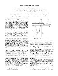
However, if measurements were made of both the electric and magnetic fields, then the<br />
near zone fields of an oscillating electric dipole, eqs. (10)-(11), would be found to be<br />
quite different from those of a magnetic dipole, eqs. (108)-(109). This is illustrated in<br />
the figure on the previous page, which plots the ratio E/H = E/B of the magnitudes<br />
of the electric and magnetic fields as a function of the distance r from the center of<br />
the dipoles.
<strong>Princeton</strong> <strong>University</strong> 2001 <strong>Ph501</strong> <strong>Set</strong> 8, Solution 2 27<br />
To distinguish between the cases of electric and magnetic dipole radiation, it suffices<br />
to measure only the polarization (i.e., the direction, but not the magnitude) of either<br />
the electric of the magnetic field vectors.
<strong>Princeton</strong> <strong>University</strong> 2001 <strong>Ph501</strong> <strong>Set</strong> 8, Solution 3 28<br />
3. The rotating dipole p can be thought of as two oscillating linear dipoles oriented 90 ◦<br />
apart in space, and phased 90 ◦ apart in time. This is conveniently summarized in<br />
complex vector notation:<br />
p = p 0 (ˆx + iŷ)e −iωt , (110)<br />
for a rotation from the +ˆx axis towards the +ŷ axis. Thus,<br />
[¨p] =¨p(t ′ = t − r/c) =−ω 2 p 0 (ˆx + iŷ)e i(kr−ωt) . (111)<br />
The radiation fields of this oscillating dipole are given by<br />
B rad =<br />
[¨p] × ˆn<br />
c 2 r<br />
= − k2 p 0 e −i(kr−ωt)<br />
(ˆx + iŷ) × ˆn<br />
r<br />
= k2 p 0 e −i(kr−ωt)<br />
(cos θ ŷ − i<br />
r<br />
ˆl), (112)<br />
E rad = B rad × ˆn = k2 p 0 e −i(kr−ωt)<br />
(cos θ<br />
r<br />
ˆl + i ŷ). (113)<br />
The time-averaged angular distribution of the radiated power is given by<br />
d 〈P 〉<br />
dΩ<br />
= c<br />
8π r2 |B rad | 2 = c<br />
8π k4 p 2 0(1 + cos 2 θ), (114)<br />
since ˆl and ŷ are orthogonal. The total radiated power is therefore<br />
〈P 〉 =<br />
∫ d 〈P 〉<br />
dΩ<br />
The total power also follows from the Larmor formula,<br />
〈P 〉 = 1 2<br />
since |¨p| = √ 2ω 2 p 0 in the present example.<br />
dΩ=2c 3 k4 p 2 0 = 2<br />
3c 3 ω4 p 2 0 . (115)<br />
2 |¨p| 2<br />
3c 3 = 2<br />
3c 3 ω4 p 2 0, (116)
<strong>Princeton</strong> <strong>University</strong> 2001 <strong>Ph501</strong> <strong>Set</strong> 8, Solution 4 29<br />
4. According to the Larmor formula, the rate of magnetic dipole radiation is<br />
dU<br />
dt = 2 3<br />
¨m 2<br />
c = 2 m 2 ω 4<br />
, (117)<br />
3 3 c 3<br />
where ω =2π/T is the angular velocity, taken to be perpendicular to the magnetic<br />
dipole moment m.<br />
The radiated power (117) is derived from a decrease in the rotational kinetic energy,<br />
U = Iω 2 /2, of the pulsar:<br />
dU<br />
dt = −Iω˙ω = 2 5 MR2 ω | ˙ω| , (118)<br />
where the moment of inertia I is taken to be that of a sphere of uniform mass density.<br />
Combining eqs. (117) and (118), we have<br />
m 2 = 3 MR 2 | ˙ω| c 3<br />
. (119)<br />
5 ω 3 Substituting ω =2π/T, and| ˙ω| =2π ∣T<br />
˙<br />
∣ /T 2 , we find<br />
m 2 = 3<br />
20π 2 MR2 T ∣ ∣ ∣Ṫ ∣ c 3 . (120)<br />
The static magnetic field B due to dipole m is<br />
so the peak field at radius R is<br />
B =<br />
3(m · ˆr)ˆr − m<br />
r 3 , (121)<br />
B = 2m R 3 . (122)<br />
Inserting this in eq. (120), the peak surface magnetic field is related by<br />
B 2 = 3<br />
MT ∣ ˙<br />
T ∣ c 3<br />
= 3 (2.8 × 10 33 )(7.5)(8 × 10 −11 )(3 × 10 10 ) 3<br />
=2.8 × 10 30 gauss 2 .<br />
5π 2 R 4 5π 2 (10 6 ) 4 (123)<br />
Thus, B peak =1.7 × 10 15 G=38B crit ,whereB crit =4.4 × 10 13 G.<br />
When electrons and photons of kinetic energies greater than 1 MeV exist in a magnetic<br />
field with B>B crit , they rapidly lose this energy via electron-positron pair creation.<br />
Kouveliotou et al. report that B peak =8× 10 14 G without discussing details of their<br />
calculation.
<strong>Princeton</strong> <strong>University</strong> 2001 <strong>Ph501</strong> <strong>Set</strong> 8, Solution 5 30<br />
5. The time-average field momentum density is given in terms of the Poynting vector as<br />
(the real part of)<br />
〈P〉 field<br />
= 〈S〉 c<br />
c 2 8π E × B⋆ . (124)<br />
Hence, the time-averaged angular momentum density is<br />
〈L〉 field<br />
= r × P field = 1<br />
8πc r × (E × B⋆ )= 1<br />
8πc r[E(ˆn · B⋆ ) − B ⋆ (ˆn · E)]. (125)<br />
writing r = rˆn.<br />
The time-average rate of radiation of angular momentum into solid angle dΩ is therefore<br />
d 〈L〉<br />
dt dΩ = cr2 〈L〉 field<br />
= 1<br />
8π r3 [E(ˆn · B ⋆ ) − B ⋆ (ˆn · E)], (126)<br />
since the angular momentum density L is moving with velocity c.<br />
The radiation fields of an oscillating electric dipole moment p including both the 1/r<br />
and 1/r 2 terms of eqs. (80) and (88) are,<br />
[(<br />
E = k ei(kr−ωt)<br />
k + i ) (<br />
p − k + 3i ) ]<br />
(ˆn · p)ˆn , (127)<br />
r r<br />
r<br />
(<br />
B = k 2 ei(kr−ωt)<br />
1+ i )<br />
(ˆn × p). (128)<br />
r kr<br />
Since ˆn · B ⋆ = 0 for this case, only the second term in eq. (126) contributes to the<br />
radiated angular momentum. We therefore find<br />
(<br />
d 〈L〉<br />
dt dΩ = r<br />
−k3 1 − i ) (<br />
(ˆn × p ⋆ ) − 2i )<br />
(ˆn · p) = ik3<br />
8π kr<br />
r<br />
4π (ˆn · p)(ˆn × p⋆ ), (129)<br />
ignoring terms in the final expression that have positive powers of r in the denominator,<br />
as these grow small at large distances.<br />
For the example of a rotating dipole moment (prob. 2),<br />
we have<br />
p = p 0 (ˆx + iŷ)e −iωt , (130)<br />
d 〈L〉<br />
dt dΩ = p 2<br />
Reik3 0<br />
4π [ˆn · (ˆx + iŷ)][ˆn × (ˆx − iŷ)] = p 2<br />
Reik3 0<br />
sin θ[cos θ ŷ + i ˆl]<br />
4π<br />
= − k3<br />
4π p2 0 sin θ ˆl. (131)<br />
To find d 〈L〉 /dt we integrate eq. (130) over solid angle. When vector ˆn is in the x-z<br />
plane, vector ˆl canbeexpressedas<br />
ˆl =cosθ ˆx − sin θ ẑ. (132)
<strong>Princeton</strong> <strong>University</strong> 2001 <strong>Ph501</strong> <strong>Set</strong> 8, Solution 5 31<br />
As we integrate over all directions of ˆn, the contributions to d 〈L〉 /dt in the x-y plane<br />
sum to zero, and only its z component survives. Hence,<br />
d 〈L〉<br />
dt<br />
∫ d 〈Lz 〉<br />
= ẑ<br />
dt dΩ<br />
= 2ck3<br />
∫<br />
k3 1<br />
dΩ=2π<br />
4π p2 0 ẑ sin 2 θdcos θ = 2k3<br />
−1<br />
3 p2 0 ẑ<br />
3ω p2 0 ẑ = 〈P 〉 ẑ, (133)<br />
ω<br />
recalling eq. (116) for the radiated power 〈P 〉. Of course, the motion described by<br />
eq. (130) has its angular momentum along the +z axis.
<strong>Princeton</strong> <strong>University</strong> 2001 <strong>Ph501</strong> <strong>Set</strong> 8, Solution 6 32<br />
6. The magnetic field radiated by a time-dependent, axially symmetric quadrupole is<br />
given by<br />
B = [ Q] ...<br />
× ˆn<br />
(134)<br />
6c 3 r<br />
where the unit vector ˆn has rectangular components<br />
ˆn =(sinθ, 0, cos θ), (135)<br />
and the quadrupole vector Q is related to the quadrupole tensor Q ij by<br />
Q i = Q ij n j . (136)<br />
The charge distribution is symmetric about the z axis, so the quadrupole moment<br />
tensor Q ij may be expressed entirely in terms of<br />
∫<br />
Q zz = ρ(3z 2 − r 2 ) dVol = −4a 2 e cos 2 ωt = −2a 2 e(1 + cos 2ωt). (137)<br />
Thus,<br />
⎛<br />
⎞<br />
−Q zz /2 0 0<br />
Q ij =<br />
⎜<br />
0 −Q zz /2 0<br />
, (138)<br />
⎟<br />
⎝<br />
⎠<br />
0 0 Q zz<br />
and the quadrupole vector can be written as<br />
(<br />
Q = − Q )<br />
zz sin θ<br />
, 0,Q zz cos θ = − Q zz<br />
2<br />
2 ˆn + 3Q zz cos θ<br />
ẑ<br />
2<br />
= a 2 e(1 + cos 2ωt)(ˆn − 3ẑ cos θ). (139)<br />
Then,<br />
[ Q] ...<br />
=8ω 3 a 2 e sin 2ωt ′ (ˆn − 3ẑ cos θ), (140)<br />
where the retarded time is t ′ = t − r/c. Hence,<br />
B = [ Q] ...<br />
× ˆn<br />
= − 4k3 a 2 e<br />
ŷ sin(2kr − 2ωt) sinθ cos θ, (141)<br />
6c 3 r r<br />
since ẑ × ˆn = ŷ sin θ. The radiated electric field is given by<br />
E = B × ˆn = − 4k3 a 2 e<br />
ˆl sin(2kr − 2ωt) sinθ cos θ, (142)<br />
r<br />
using ŷ × ˆn = ˆl.<br />
As we are not using complex notation, we revert to the basic definitions to find that<br />
the time-averaged angular distribution of radiated power is<br />
d 〈P 〉<br />
dΩ<br />
= r2 〈S〉·ˆn = cr2<br />
4π 〈E × B · ˆn〉 = 2ck6 a 4 e 2<br />
π<br />
since ˆl × ŷ = ˆn. This integrates to give<br />
〈P 〉 =2π<br />
∫ 1<br />
−1<br />
sin 2 θ cos 2 θ, (143)<br />
d 〈P 〉<br />
dΩ d cos θ = 16ck6 a 4 e 2<br />
. (144)<br />
15
<strong>Princeton</strong> <strong>University</strong> 2001 <strong>Ph501</strong> <strong>Set</strong> 8, Solution 7 33<br />
7. Since the charge is assumed to rotate with constant angular velocity, the magnetic<br />
moment it generates is constant in time, and there is no magnetic dipole radiation.<br />
Hence, we consider only electric quadrupole radiation in addition to the electric dipole<br />
radiation. The radiated fields are therefore<br />
B =<br />
[¨p] × ˆn<br />
c 2 r<br />
+ [ Q] ...<br />
× ˆn<br />
, E = B × ˆn. (145)<br />
6c 3 r<br />
The electric dipole radiation fields are given by eqs. (112) and 113) when we write<br />
p 0 = ae.<br />
The present charge distribution is not azimuthally symmetric about any fixed axis, so<br />
we must evaluate the full quadrupole tensor,<br />
Q ij = e(3r i r j − r 2 δ ij ). (146)<br />
to find the components of the quadrupole vector Q. The position vector of the charge<br />
has components<br />
r i =(a cos ωt, a sin ωt, 0), (147)<br />
so the nonzero components of Q ij are<br />
Q xx = e(3x 2 − r 2 )=a 2 e(3 cos 2 ωt − 1) = a2 e<br />
(1 + 3 cos 2ωt),<br />
2<br />
(148)<br />
Q yy = e(3y 2 − r 2 )=a 2 e(3 sin 2 ωt − 1) = a2 e<br />
(1 − 3cos2ωt),<br />
2<br />
(149)<br />
Q zz = −er 2 = −a 2 e, (150)<br />
Q xy = Q yx =3exy =3a 2 e sin ωt cos ωt = 3a2 e<br />
sin 2ωt.<br />
2<br />
(151)<br />
Only the time-dependent part of Q ij contributes to the radiation, so we write<br />
⎛<br />
⎞<br />
cos 2ωt sin 2ωt 0<br />
Q ij (time dependent) = 3a2 e<br />
2 ⎜ sin 2ωt − cos 2ωt 0<br />
.<br />
⎟<br />
⎝<br />
⎠<br />
0 0 0<br />
(152)<br />
The unit vector ˆn towards the observer has components given in eq. (135), so the<br />
time-dependent part of the quadrupole vector Q has components<br />
Thus,<br />
Q i = Q ij n j = 3a2 e<br />
(cos 2ωt sin θ, sin 2ωt sin θ, 0). (153)<br />
2<br />
[ ...<br />
Q i ]= ...<br />
Q i (t ′ = t − r/c) =−12a 2 eω 3 sin θ(sin(2kr − 2ωt), cos(2kr − 2ωt), 0). (154)<br />
It is preferable to express this vector in terms of the orthonormal triad ˆn, ŷ, and<br />
ˆl = ŷ × ˆn, bynotingthat<br />
ˆx = ˆn sin θ − ˆl cos θ. (155)
<strong>Princeton</strong> <strong>University</strong> 2001 <strong>Ph501</strong> <strong>Set</strong> 8, Solution 7 34<br />
Hence,<br />
[ Q] ...<br />
=−12a 2 eω 3 sin θ(ˆn sin θ sin(2kr − 2ωt) −ˆl cos θ sin(2kr − 2ωt)+ŷ cos(2kr − 2ωt)).<br />
(156)<br />
The field due to electric quadrupole radiation are therefore<br />
B E2 = [ Q] ...<br />
× ˆn<br />
= − 2a2 ek 3<br />
sin θ(ˆl cos(2kr − 2ωt)+ŷ cos θ sin(2kr − 2ωt)),(157)<br />
6c 3 r r<br />
E E2 = B E2 × ˆn = 2a2 ek 3<br />
sin θ(ŷ cos(2kr − 2ωt) −<br />
r<br />
ˆl cos θ sin(2kr − 2ωt)). (158)<br />
The angular distribution of the radiated power can be calculated from the combined<br />
electric dipole and electric quadrupole fields, and will include a term ∝ k 4 due only to<br />
dipole radiation as found in prob. 2, a term ∝ k 6 due only to quadrupole radiation,<br />
and a complicated cross term ∝ k 5 due to both dipole and quadrupole field. Here, we<br />
only display the term due to the quadrupole fields by themselves:<br />
d 〈P E2 〉<br />
dΩ<br />
which integrates to give<br />
= cr2<br />
4π 〈E E2 × B E2 · ˆn〉 = ca4 e 2 k 6<br />
(1 − cos 4 θ), (159)<br />
2π<br />
∫ 1 d 〈P 〉<br />
〈P E2 〉 =2π<br />
−1 dΩ d cos θ = 8ca4 e 2 k 6<br />
. (160)<br />
5
<strong>Princeton</strong> <strong>University</strong> 2001 <strong>Ph501</strong> <strong>Set</strong> 8, Solution 8 35<br />
8. a) The dominant energy loss is from electric dipole radiation, which obeys eq. (25),<br />
dU<br />
dt = −〈P E1〉 = − 2a2 e 2 ω 4<br />
. (161)<br />
3c 3<br />
For an electron of charge −e and mass m in an orbit of radius a about a fixed nucleus<br />
of charge +e, F = ma tells us that<br />
e 2<br />
a 2 = mv2 a = mω2 a, (162)<br />
so that<br />
ω 2 =<br />
e2<br />
ma , (163)<br />
3<br />
and also the total energy (kinetic plus potential) is<br />
U = − e2<br />
a + 1 2 mv2 = − e2<br />
2a<br />
(164)<br />
Using eqs. (163) and (164) in (161), we have<br />
dU<br />
dt = e2<br />
2a ȧ = − 2e6<br />
2 3a 4 m 2 c , (165)<br />
3<br />
or<br />
a 2 ȧ = 1 da 3<br />
3 dt = − 4e4<br />
3m 2 c = −4 3 3 r2 0c, (166)<br />
where r 0 = e 2 /mc 2 is the classical electron radius. Hence,<br />
a 3 = a 3 0 − 4r 2 0ct. (167)<br />
The time to fall to the origin is<br />
t fall = a3 0<br />
4r 2 0c . (168)<br />
With r 0 =2.8 × 10 −13 cm and a 0 =5.3 × 10 −9 cm, t fall =1.6 × 10 −11 s.<br />
This is of the order of magnitude of the lifetime of an excited hydrogen atom, but the<br />
ground state appears to have infinite lifetime.<br />
This classical puzzle is pursued further in prob. 7.<br />
b) The analog of the quadrupole factor ea 2 in prob. 5 for masses m 1 and m 2 in circular<br />
orbits with distance a between them is m 1 r1 2 + m 2r2 2,wherer 1 and r 2 are measured<br />
from the center of mass. That is,<br />
m 1 r 1 = m 2 r 2 , and r 1 + r 2 = a, (169)<br />
so that<br />
r 1 =<br />
m 2<br />
m 1 + m 2<br />
a, r 2 =<br />
m 1<br />
m 1 + m 2<br />
a, (170)
<strong>Princeton</strong> <strong>University</strong> 2001 <strong>Ph501</strong> <strong>Set</strong> 8, Solution 8 36<br />
and the quadrupole factor is<br />
m 1 r 2 1 + m 2 r 2 2 = m 1m 2<br />
m 1 + m 2<br />
a 2 . (171)<br />
We are then led by eq. (26) to say that the power in gravitational quadrupole radiation<br />
is<br />
P G2 = 8 ( )<br />
G m1 m 2 2<br />
a 4 ω 6 . (172)<br />
5 c 5 m 1 + m 2<br />
We insert a single factor of Newton’s constant G in this expression, since it has dimensions<br />
of mass 2 ,andGm 2 is the gravitational analog of the square of the electric charge<br />
in eq. (26).<br />
We note that a general relativity calculation yields a result a factor of 4 larger than<br />
eq. (172):<br />
P G2 = 32 ( )<br />
G m1 m 2 2<br />
a 4 ω 6 . (173)<br />
5 c 5 m 1 + m 2<br />
To find t fall due to gravitational radiation, we follow the argument of part a):<br />
Gm 1 m 2 v1<br />
2 = m<br />
a 2 1 = m 1 ω 2 v2<br />
2 r 1 = m 2 , (174)<br />
r 1 r 2<br />
so that<br />
ω 2 = G(m 1 + m 2 )<br />
, (175)<br />
a 3<br />
and also the total energy (kinetic plus potential) is<br />
U = − Gm 1m 2<br />
a<br />
Using eqs. (175) and (176) in (173), we have<br />
+ 1 2 m 1v 2 1 + 1 2 m 2v 2 2 = −Gm 1m 2<br />
2a<br />
(176)<br />
dU<br />
dt = Gm 1m 2<br />
ȧ = − 32G4 m 2 1m 2 2(m 1 + m 2 )<br />
, (177)<br />
2a 2 5a 5 c 5<br />
or<br />
a 3 ȧ = 1 da 4<br />
4 dt = m 1 m 2 (m 1 + m 2 )<br />
−64G3 . (178)<br />
5c 5<br />
Hence,<br />
a 4 = a 4 0 − 256G3 m 1 m 2 (m 1 + m 2 )<br />
t. (179)<br />
5c 5<br />
The time to fall to the origin is<br />
t fall =<br />
5a 4 0c 5<br />
256G 3 m 1 m 2 (m 1 + m 2 ) . (180)<br />
For the Earth-Sun system, a 0 =1.5 × 10 13 cm, m 1 =6× 10 27 gm, m 2 =2× 10 33 cm,<br />
and G =6.7 × 10 −10 cm 2 /(g-s 2 ), so that t fall ≈ 1.5 × 10 36 s ≈ 5 × 10 28 years!
<strong>Princeton</strong> <strong>University</strong> 2001 <strong>Ph501</strong> <strong>Set</strong> 8, Solution 9 37<br />
9. The solution given here follows the succinct treatment by Landau, Classical Theory of<br />
Fields, sec. 74.<br />
For charges in steady motion at angular frequency ω in a ring of radius a, the current<br />
density J is periodic with period 2π/ω, so the Fourier analysis (34) at the retarded<br />
time t ′ can be evaluated via the usual approximation that r ≈ R − r ′ · ˆn, whereR is<br />
the distance from the center of the ring to the observer, r ′ points from the center of<br />
the ring to the electron, and ˆn is the unit vector pointing from the center of the ring<br />
to the observer. Then,<br />
[J] = J(r ′ ,t ′ = t − r/c) = ∑ m<br />
J m (r ′ )e −imω(t−R/c+r′·ˆn/c<br />
= ∑ m<br />
e im(kR−ωt) J m (r ′ )e −imωr′·ˆn/c , (181)<br />
where k = ω/c.<br />
We first consider a single electron, whose azimuth varies as φ = ωt + φ 0 ,andwhose<br />
velocity is, of course, v = aω. The current density of a point electron of charge e can<br />
be written in a cylindrical coordinate system (ρ, φ, z) (with volume element ρdρ dφ dz)<br />
using Dirac delta functions as<br />
J = ρ charge v ˆφ = evδ(ρ − a)δ(z)δ(ρ(φ − ωt − φ 0 ))ˆφ. (182)<br />
The Fourier components J m are given by<br />
J m = 1 T<br />
∫ T<br />
0<br />
J(r,t)e imt dt = evδ(ρ − a)δ(z) eim(φ−φ 0)<br />
ˆφ. (183)<br />
ρωT<br />
Also,<br />
r ′ = ρ(cos φ ˆx+sinφ ŷ), ˆn =sinθ ˆx+cosθ ẑ, and ˆφ = − sin φ ˆx+cosφ ŷ. (184)<br />
Using eqs. (183) and (184) in (181) and noting that ωT =2π, we find<br />
[J] = ev ∑<br />
e im(kR−ωt) e im(φ−φ 0−ωρ sin θ cos φ/c) δ(ρ − a)δ(z)ˆφ. (185)<br />
2πρ<br />
Inserting this in eq. (33), we have<br />
m<br />
A ≈ 1 ∫<br />
[J]ρ dρdφdz=<br />
ev ∑<br />
∫ 2π<br />
e im(kR−ωt−φ 0 ) e im(φ−ωa sin θ cos φ/c) ˆφ dφ<br />
cR<br />
2πcR m<br />
0<br />
= ∑ A m e −imωt , (186)<br />
m<br />
so that the Fourier components of the vector potential are<br />
A m =<br />
ev<br />
∫ 2π<br />
2πcR eim(kR−φ 0 ) e im(φ−v sin θ cos φ/c) (− sin φ ˆx +cosφ ŷ) dφ. (187)<br />
0
<strong>Princeton</strong> <strong>University</strong> 2001 <strong>Ph501</strong> <strong>Set</strong> 8, Solution 9 38<br />
The integrals yield Bessel functions with the aid of the integral representation (40).<br />
The ŷ part of eq. (187) can be found by taking the derivative of this relation with<br />
respect to z:<br />
∫ 2π<br />
J m ′ (z) =−im+1 e imφ−iz cos φ cos φdφ, (188)<br />
2π 0<br />
For the ˆx part of eq. (187) we play the trick<br />
0 =<br />
∫ 2π<br />
= m<br />
0<br />
∫ 2π<br />
so that<br />
∫<br />
1 2π<br />
e imφ−iz cos φ sin φdφ= − m 2π 0<br />
z<br />
0<br />
e i(mφ−z cos φ) d(mφ − z cos φ)<br />
∫ 2π<br />
e imφ−iz cos φ dφ + z e imφ−iz cos φ sin φdφ, (189)<br />
0<br />
∫<br />
1 2π<br />
e imφ−iz cos φ dφ = − m<br />
2π 0<br />
i m z J m(z). (190)<br />
Using eqs. (188) and (190) with z = mv sin θ/c in (187) we have<br />
A m = ev<br />
(<br />
cR eim(kR−φ 0 ) 1<br />
i m v sin θ/c J m(mv sin θ/c) ˆx − 1<br />
)<br />
i J m(mv ′ sin θ/c) ŷ . (191)<br />
m+1<br />
We skip the calculation of the electric and magnetic fields from the vector potential,<br />
and proceed immediately to the angular distribution of the radiated power according<br />
to eq. (39),<br />
dP m<br />
dΩ = cR2<br />
2π |imkˆn × A m| 2 = ck2 m 2 R 2<br />
|ˆn × A m | 2<br />
2π<br />
= ck2 m 2 R 2 (<br />
cos 2 θ |A m,x | 2 + |A m,y | 2)<br />
2π<br />
= ce2 k 2 m 2<br />
2π<br />
(<br />
)<br />
cot 2 θJm(mv 2 sin θ/c)+ v2<br />
c J ′ 2<br />
2 m (mv sin θ/c) . (192)<br />
The present interest in this result is for v/c ≪ 1, but in fact it holds for any value of<br />
v/c. As such, it can be used for a detailed discussion of the radiation from a relativistic<br />
electron that moves in a circle, which emits so-called synchrotron radiation. This topic<br />
is discussed further in Lecture 20 of the Notes.<br />
We now turn to the case of N electrons uniformly spaced around the ring. The initial<br />
azimuth of the nth electron can be written<br />
φ n = 2πn<br />
N . (193)<br />
The mth Fourier component of the total vector potential is simply the sum of components<br />
(191) inserting φ n in place of φ 0 :<br />
A m =<br />
N∑<br />
n=1<br />
= eveimkR<br />
cR<br />
ev<br />
cR eim(kR−φ n)<br />
(<br />
(<br />
1<br />
i m v sin θ/c J m(mv sin θ/c)ˆx − 1<br />
)<br />
i J m(mv ′ sin θ/c)ŷ<br />
m+1<br />
1<br />
i m v sin θ/c J m(mv sin θ/c)ˆx − 1<br />
i J m(mv ′ sin θ/c)ŷ<br />
m+1<br />
) N ∑<br />
(194)<br />
e −i2πmn/N .<br />
n=1
<strong>Princeton</strong> <strong>University</strong> 2001 <strong>Ph501</strong> <strong>Set</strong> 8, Solution 9 39<br />
This sum vanishes unless m is a multiple of N, in which case the sum is just N. The<br />
lowest nonvanishing Fourier component has order N, and the radiation is at frequency<br />
Nω. We recognize this as Nth-order multipole radiation, whose radiated power follows<br />
from eq. (192) as<br />
dP N<br />
dΩ = ce2 k 2 N 2 (<br />
)<br />
cot 2 θJ 2<br />
2π<br />
N(Nvsin θ/c)+ v2<br />
c J ′ 2<br />
2 N (Nvsin θ/c) . (195)<br />
For large N but v/c ≪ 1 we can use the asymptotic expansion (41), and its derivative,<br />
J ′ m(mx) ≈ (ex/2)m √<br />
2πm x<br />
(m ≫ 1,x≪ 1), (196)<br />
to write eq. (195) as<br />
dP N<br />
dΩ ≈<br />
ce2 k 2 ( )<br />
N e v 2N<br />
4π 2 sin 2 θ 2 c sin θ (1 + cos 2 θ) ≪ N dP E1<br />
dΩ<br />
(N ≫ 1,v/c≪ 1). (197)<br />
In eqs. (196) and (197) the symbol e inside the parentheses is not the charge but rather<br />
the base of natural logarithms, 2.718...<br />
For currents in, say, a loop of copper wire, v ≈ 1 cm/s, so v/c ≈ 10 −10 , while N ≈ 10 23 .<br />
The radiated power predicted by eq. (197) is extraordinarily small!<br />
Note, however, that this nearly complete destructive interference depends on the electrons<br />
being uniformly distributed around the ring. Suppose instead that they were<br />
distributed with random azimuths φ n . Then the square of the magnetic field at order<br />
m has the form<br />
2<br />
|B m | 2 N∑<br />
∝<br />
e −imφ n<br />
= N + ∑ e −im(φ l −φ n ) = N. (198)<br />
∣<br />
∣<br />
l≠n<br />
n=1<br />
Thus, for random azimuths the power radiated by N electrons (at any order) is just<br />
N times that radiated by one electron.<br />
If the charge carriers in a wire were localized to distances much smaller than their<br />
separation, radiation of “steady” currents could occur. However, in the quantum view<br />
of metallic conduction, such localization does not occur.<br />
The random-phase approximation is relevant for electrons in a so-called storage ring,<br />
for which the radiated power is a major loss of energy – or source of desirable photon<br />
beams of synchrotron radiation, depending on one’s point of view. We cannot expound<br />
here on the interesting topic of the “formation length” for radiation by relativistic<br />
electrons, which length sets the scale for interference of multiple electrons. See, for<br />
example, http://puhep1.princeton.edu/~mcdonald/accel/weizsacker.pdf
<strong>Princeton</strong> <strong>University</strong> 2001 <strong>Ph501</strong> <strong>Set</strong> 8, Solution 10 40<br />
10. We repeat the derivation of Prob. 1, this time emphasizing the advanced fields.<br />
The advanced vector potential for the point electric dipole p = p 0 e −iωt located at the<br />
origin is<br />
A E1,adv = {ṗ}<br />
cr<br />
where k = ω/c.<br />
= ṗ(t′ = t + r/c)<br />
cr<br />
= −iω e−i(kr+ωt)<br />
cr<br />
We obtain the magnetic field by taking the curl of eq. (199),<br />
B E1,adv = ∇ × A E1,adv = −ik∇ e−i(kr+ωt)<br />
r<br />
= k 2 e−i(kr+ωt)<br />
r<br />
p 0 = −ik e−i(kr+ωt)<br />
p 0 , (199)<br />
r<br />
× p 0 = −ik e−i(kr+ωt)<br />
−ikˆn − ˆn × p 0<br />
r<br />
r<br />
(<br />
−1+ i )<br />
ˆn × p 0 . (200)<br />
kr<br />
Then,<br />
E E1,adv = i [ (<br />
ik<br />
k ∇ × B E1,adv = −∇ × e −i(kr+ωt) r + 1 ) ]<br />
r × p 2 r 3 0<br />
( ik<br />
= −∇e −i(kr+ωt) r + 1 )<br />
( ik<br />
× (r × p 2 r 3 0 ) − e −i(kr+ωt) r + 1 )<br />
∇ × (r × p 2 r 3 0 )<br />
[ (<br />
= e −i(kr+ωt) − k2 ik<br />
r +3 r + 1 )]<br />
( ik<br />
ˆn × (ˆn × p 2 r 3 0 )+2p 0 e −i(kr+ωt) r + 1 )<br />
2 r 3<br />
{[ (<br />
= e −i(kr+ωt) − k2 ik<br />
r +3 r + 1 )]<br />
(p 2 r 3 0 · ˆn)ˆn +<br />
[ k<br />
2<br />
The retarded fields due to a point dipole −p are, from Prob. 1,<br />
B E1,ret = −k 2 ei(kr−ωt)<br />
r<br />
{[ k<br />
E E1,ret = e i(kr−ωt) 2<br />
(<br />
1+ i )<br />
kr<br />
(<br />
)<br />
r − ik<br />
r 2 − 1 r 3 ]<br />
p 0<br />
}<br />
. (201)<br />
ˆn × p 0 , (202)<br />
( ik<br />
r +3 r − 1 )]<br />
[ k<br />
2<br />
(p 2 r 3 0 · ˆn)ˆn −<br />
r + ik<br />
r − 1 ] }<br />
p 2 r 3 0 .(203)<br />
We now consider the superposition of the fields (200)-(203) inside a conducting sphere<br />
of radius a. The spatial part of the total electric field is then<br />
[( k<br />
2<br />
E E1 =<br />
r − 3 )<br />
(e ikr − e −ikr )+3 ik<br />
]<br />
r 3 r 2 (eikr + e −ikr ) (p 0 · ˆn)ˆn<br />
[( k<br />
2<br />
−<br />
r − 1 )<br />
(e ikr − e −ikr )+ ik<br />
]<br />
r 3 r 2 (eikr + e −ikr ) p 0<br />
[( k<br />
2<br />
= 2i<br />
r − 3 )<br />
sin kr +3 k ]<br />
r 3 r cos kr (p 2 0 · ˆn)ˆn<br />
[( k<br />
2<br />
−2i<br />
r − 1 )<br />
sin kr + k ]<br />
r 3 r cos kr p 2 0 . (204)
<strong>Princeton</strong> <strong>University</strong> 2001 <strong>Ph501</strong> <strong>Set</strong> 8, Solution 10 41<br />
Remarkably, this electric field is finite at the origin, although each of the fields (201)<br />
and (203) diverges there. We also recognize that this electric field could be expressed<br />
in terms of the so-called spherical Bessel functions,<br />
j 0 (x) = sin x<br />
x , j 1(x) = sin x − cos x<br />
3<br />
x 2 x , j 2(x) =(<br />
x − 1 )<br />
sin x − 3cosx , ... (205)<br />
3 x x 2<br />
An expansion of the spherical cavity field in terms of spherical Bessel functions occurs<br />
“naturally” when we use the more standard approach to this problem, seeking solutions<br />
to the Helmholtz wave equation via separation of variables in spherical coordinates. See<br />
Electromagnetic Theory by J.A. Stratton (McGraw-Hill, New York, 1941) for details<br />
of this method.<br />
Because the sum of the magnetic fields (200) and (202) is purely transverse, this cavity<br />
mode is called a TM mode.<br />
The boundary conditions at the surface of the sphere are that the radial component<br />
of the magnetic field and the transverse component of the electric field must vanish.<br />
Since the magnetic fields (200) and (202) are transverse at any radius, we examine the<br />
electric field at r = a. Of the terms in eq. (204), only those in p 0 have transverse<br />
components, so the boundary condition is<br />
0= k ( k<br />
2<br />
a cos ka +sinka 2 a − 1 )<br />
, (206)<br />
a 3<br />
or<br />
cot ka = 1 − ka ⇒ ka =2.744. (207)<br />
ka<br />
In case of a point magnetic dipole m = m 0 e −iωt at the origin, the fields have the same<br />
form as for an electric dipole, but with E and B interchanged. That is, the advanced<br />
fields would be<br />
E M1,adv = k 2 e−i(kr+ωt)<br />
r<br />
{[<br />
B M1,adv = e −i(kr+ωt)<br />
(<br />
−1+ i )<br />
kr<br />
(<br />
− k2 ik<br />
r +3 r + 1 )]<br />
(m 2 r 3 0 · ˆn)ˆn +<br />
and the retarded field due to magnetic dipole −m would be<br />
E M1,ret = −k 2 ei(kr−ωt)<br />
r<br />
{[ k<br />
B M1,ret = e i(kr−ωt) 2<br />
(<br />
1+ i )<br />
kr<br />
ˆn × m 0 , (208)<br />
[ k<br />
2<br />
r − ik<br />
r − 1 ] }<br />
m 2 r 3 0 (209) ,<br />
ˆn × m 0 , (210)<br />
( ik<br />
r +3 r − 1 )]<br />
[ k<br />
2<br />
(m 2 r 3 0 · ˆn)ˆn −<br />
r + ik<br />
r − 1 ] }<br />
m 2 r 3 0 .(211)<br />
If the advanced and retarded magnetic dipole fields are superposed inside a spherical<br />
cavity of radius a, the condition that the transverse electric field vanish at the<br />
conducting surface is<br />
[<br />
0=e ika 1+ i ] [<br />
+ e −ika 1 − i ] [<br />
=2 cos ka −<br />
ka<br />
ka<br />
]<br />
sin ka<br />
, (212)<br />
ka
<strong>Princeton</strong> <strong>University</strong> 2001 <strong>Ph501</strong> <strong>Set</strong> 8, Solution 10 42<br />
or<br />
tan ka = ka ⇒ ka =4.493. (213)<br />
The electric field of this mode is purely transverse, so it is called a TE mode.<br />
Clearly, other modes of a spherical cavity can be found by superposing the advanced<br />
and retarded fields due to higher multipoles at the origin.
<strong>Princeton</strong> <strong>University</strong> 2001 <strong>Ph501</strong> <strong>Set</strong> 8, Solution 11 43<br />
11. This problem is due to D. Iwanenko and I. Pomeranchuk, On the Maximal Energy<br />
Attainable in a Betatron, Phys.Rev.65, 343 (1944). 9<br />
The electron is held in its circular orbit by the Lorentz force due to the field B.<br />
Newton’s law, F = ma, for this circular motion can be written<br />
F = γma = γmv2<br />
R = ev B. (214)<br />
c<br />
For a relativistic electron, v ≈ c, sowehave<br />
γ ≈ eRB<br />
mc . (215)<br />
2<br />
The electron is being accelerated by the electric field that is induced by the changing<br />
magnetic flux. Applying the integral form of Faraday’s law to the circle of radius R,<br />
we have (ignoring the sign)<br />
and hence,<br />
2πRE φ = ˙Φ<br />
c = πR2 Ḃ ave<br />
, (216)<br />
c<br />
E φ = RḂave<br />
, (217)<br />
2c<br />
The rate of change of the electron’s energy E due to E φ is<br />
dE<br />
dt = F · v ≈ ecE φ = eRḂave<br />
, (218)<br />
2<br />
Since E = γmc 2 ,wecanwrite<br />
˙γmc 2 = eRḂave , (219)<br />
2<br />
which integrates to<br />
γ = eRB ave<br />
2mc . (220)<br />
2<br />
Comparing with eq. (215), we find the required condition on the magnetic field:<br />
B = B ave<br />
2 . (221)<br />
As the electron accelerates it radiates energy at rate given by the Larmor formula in<br />
the rest frame of the electron,<br />
dE ⋆<br />
dt ⋆<br />
⋆2<br />
= −2e2¨p<br />
3c 3<br />
= − 2e2 a ⋆2<br />
3c 3 (222)<br />
Because E and t are both the time components of 4-vectors their transforms from<br />
the rest frame to the lab frame have the same form, and the rate dE/dt is invariant.<br />
9 http://puhep1.princeton.edu/~mcdonald/examples/EM/iwanenko_pr_65_343_44.pdf
<strong>Princeton</strong> <strong>University</strong> 2001 <strong>Ph501</strong> <strong>Set</strong> 8, Solution 11 44<br />
However, acceleration at right angles to velocity transforms according to a ⋆ = γ 2 a.<br />
Hence, the rate of radiation in the lab frame is<br />
dE<br />
dt = γ 4 a 2<br />
−2e2 = − 2e4 γ 2 B 2<br />
3c 3 3m 2 c , (223)<br />
3<br />
using eq. (214) for the acceleration a.<br />
The maximal energy of the electrons in the betatron obtains when the energy loss (223)<br />
cancels the energy gain (218), i.e., when<br />
and<br />
γ max =<br />
eRḂave<br />
2<br />
√<br />
√<br />
3m 2 c 3 RḂ ave 3R Ḃ ave B crit<br />
=<br />
4e 3 B 2 4αc B B<br />
= 2e4 γ 2 maxB 2<br />
3m 2 c 3 , (224)<br />
√<br />
3R<br />
≈ B crit<br />
4αcτ B , (225)<br />
where α = e 2 /¯hc =1/137 is the fine structure constant, B crit = m 2 c 3 /e¯h =4.4×10 13 G<br />
is the so-called QED critical field strength, and τ is the characteristic cycle time of the<br />
betatron such that Ḃ ave = B/τ. For example, with R =1m,τ =0.03 sec (30 Hz),<br />
and B =10 4 G, we find that γ max ≈ 200, or E max ≈ 100 MeV.<br />
We have ignored the radiation due to the longitudinal acceleration of the electron,<br />
since in the limiting case this acceleration ceases.
<strong>Princeton</strong> <strong>University</strong> 2001 <strong>Ph501</strong> <strong>Set</strong> 8, Solution 12 45<br />
12. Since the dipole is much less than a wavelength away from the conducting plane, the<br />
fields between the dipole and the plane are essentially the instantaneous static fields.<br />
Thus, charges arranges themselves on the plane as if there were an image dipole at<br />
distance d on the other side of the plane. The radiation from the moving charges on<br />
the plan is effectively that due to the oscillating image dipole. A distant observer sees<br />
the sum of the radiation fields from the dipole and its image.<br />
The image dipole is inverted with respect to the original, i.e., the two dipoles are 180 ◦<br />
out of phase.<br />
Furthermore, there is a difference s in path length between the two dipole and the<br />
distant observer at angles (θ, φ). We first calculate in a spherical coordinate system<br />
with z axis along the first dipole, and x axis pointing from the plane to that dipole.<br />
Then the path difference is<br />
s =2dˆx · ˆn =2d sin θ cos φ. (226)<br />
This path difference results in an additional phase difference δ between the fields from<br />
the two dipoles at the observer, in the amount<br />
δ =2π s λ = 4πd<br />
λ<br />
sin θ cos φ. (227)<br />
If we label the electric fields due to the original and image dipoles as E 1 and E 2 ,<br />
respectively, then the total field is<br />
and, recalling eq. (46), the power radiated is<br />
E = E 1 + E 2 = E 1 (1 − e iδ ), (228)<br />
dP<br />
dΩ = |E|2 dP ∣ 1 ∣∣1 ∣<br />
|E 1 | 2 dΩ = − e<br />
iδ 2<br />
∣ A sin 2 θ =2A sin 2 θ(1 − cos δ) =4A sin 2 θ sin 2 δ/2<br />
= 4A sin 2 θ sin 2 Δ, (229)<br />
where<br />
Δ= δ 2 = 2πd<br />
λ<br />
sin θ cos φ. (230)<br />
Suppose we had chosen to use a spherical coordinate system (r, θ ′ ,φ ′ )withthez ′ axis<br />
pointing from the plane to dipole 1, and the x ′ axis parallel to dipole 1. Then the
<strong>Princeton</strong> <strong>University</strong> 2001 <strong>Ph501</strong> <strong>Set</strong> 8, Solution 12 46<br />
phase difference would have the simple form<br />
Δ= δ 2 = π λ 2d ẑ′ · ˆn = 2πd<br />
λ cos θ′ , (231)<br />
but the factor sin 2 θ would now become<br />
sin 2 θ = n 2 x + n2 y = n2 z ′ + n2 y ′ =cos2 θ ′ +sin 2 θ ′ cos 2 φ ′ =1− sin 2 θ ′ sin 2 φ ′ . (232)<br />
If d = λ/4, then<br />
( )<br />
dP<br />
π<br />
dΩ =4A sin2 θ sin 2 2 sin θ cos φ . (233)<br />
In the “side” view, φ = 0, so the pattern has shape<br />
( ) π<br />
sin 2 θ sin 2 2 sin θ (side view), (234)<br />
while in the “top” view, θ = π/2 and the shape is<br />
sin 2 ( π<br />
2 cos φ )<br />
(top view). (235)<br />
This pattern has a single lobe in the forward hemisphere, as illustrated below:<br />
If instead, d = λ/2, then<br />
dP<br />
dΩ =4A sin2 θ sin 2 (π sin θ cos φ) . (236)<br />
In the “side” view, φ = 0, so the pattern has shape<br />
sin 2 θ sin 2 (π sin θ) (side view), (237)
<strong>Princeton</strong> <strong>University</strong> 2001 <strong>Ph501</strong> <strong>Set</strong> 8, Solution 12 47<br />
while in the “top” view, θ = π/2 and the shape is<br />
sin 2 (π cos φ) (top view). (238)<br />
This pattern does not radiate along the line from the plane to the dipole, as illustrated<br />
below:<br />
b) If the electric dipole is aligned with the line from the plane to the dipole, its image<br />
has the same orientation.<br />
The only phase difference between the radiation fields of the dipole and its image is<br />
that due to the path difference δ, whose value has been given in eqs. (230) and (231).<br />
It is simpler to use the angles (θ ′ ,φ ′ ) in this case, since the radiation pattern of a single<br />
dipole varies as sin 2 θ ′ . Then,<br />
and, recalling eq. (46), the power radiated is<br />
E = E 1 + E 2 = E 1 (1 + e iδ ), (239)<br />
dP<br />
dΩ = |E|2 dP ∣ 1 ∣∣1+e ∣<br />
|E 1 | 2 dΩ = iδ 2<br />
∣ A sin 2 θ ′ =2A sin 2 θ ′ (1 + cos δ) =4A sin 2 θ ′ cos 2 δ/2<br />
= 4A sin 2 θ ′ cos 2 Δ, (240)<br />
with<br />
Δ= δ 2 = 2πd<br />
λ cos θ′ . (241)<br />
This radiation pattern is axially symmetric about the line from the plane to the dipole.
<strong>Princeton</strong> <strong>University</strong> 2001 <strong>Ph501</strong> <strong>Set</strong> 8, Solution 12 48<br />
If d = λ/4, then<br />
( )<br />
dP<br />
π<br />
dΩ =4A sin2 θ ′ cos 2 2 cos θ′ . (242)<br />
This pattern is a flattened version of the “donut” pattern sin 2 θ ′ , as illustrated below:<br />
If instead, d = λ/2, then<br />
dP<br />
dΩ =4A sin2 θ ′ cos 2 (π cos θ ′ ) . (243)<br />
This pattern has a forward lobe for θ ′
<strong>Princeton</strong> <strong>University</strong> 2001 <strong>Ph501</strong> <strong>Set</strong> 8, Solution 12 49<br />
and, recalling eq. (46), the power radiated is<br />
dP<br />
dΩ = |E|2 dP ∣ 1 ∣∣1+e ∣<br />
|E 1 | 2 dΩ = iδ 2<br />
∣ A sin 2 θ =2A sin 2 θ(1 + cos δ) =4A cos 2 θ sin 2 δ/2<br />
= 4A sin 2 θ cos 2 Δ, (245)<br />
where<br />
Δ= δ 2 = 2πd<br />
λ<br />
sin θ cos φ. (246)<br />
If d = λ/4, then<br />
( )<br />
dP<br />
π<br />
dΩ =4A sin2 θ cos 2 2 sin θ cos φ . (247)<br />
In the “side” view, φ = 0, so the pattern has shape<br />
( ) π<br />
sin 2 θ cos 2 2 sin θ (side view), (248)<br />
while in the “top” view, θ = π/2 and the shape is<br />
( ) π<br />
cos 2 2 cos φ (top view). (249)<br />
This pattern, shown below, is somewhat similar to that of part a) for d = λ/2.<br />
If instead, d = λ/2, then<br />
dP<br />
dΩ =4A sin2 θ cos 2 (π sin θ cos φ) . (250)<br />
In the “side” view, φ = 0, so the pattern has shape<br />
while in the “top” view, θ = π/2 and the shape is<br />
sin 2 θ cos 2 (π sin θ) (side view), (251)<br />
cos 2 (π cos φ) (top view). (252)<br />
This pattern, shown below, is somewhat similar to that of part b) for d = λ/2.
<strong>Princeton</strong> <strong>University</strong> 2001 <strong>Ph501</strong> <strong>Set</strong> 8, Solution 12 50<br />
Finally, we consider the case of a magnetic dipole aligned with the line from the plane<br />
to the dipole, in which case its image has the opposite orientation.<br />
As in part b), the only phase difference between the radiation fields of the dipole and<br />
its image is that due to the path difference δ, whose value has been given in eqs. (230)<br />
and (231). We use the angles (θ ′ ,φ ′ ) in this case, since the radiation pattern of a single<br />
dipole varies as sin 2 θ ′ . Then,<br />
and, recalling eq. (46), the power radiated is<br />
E = E 1 + E 2 = E 1 (1 − e iδ ), (253)<br />
dP<br />
dΩ = |E|2 dP ∣ 1 ∣∣1 ∣<br />
|E 1 | 2 dΩ = − e<br />
iδ 2<br />
∣ A sin 2 θ ′ =2A sin 2 θ ′ (1 − cos δ) =4A sin 2 θ ′ sin 2 δ/2<br />
= 4A sin 2 θ ′ sin 2 Δ, (254)<br />
with<br />
Δ= δ 2 = 2πd<br />
λ cos θ′ . (255)<br />
This radiation pattern is axially symmetric about the line from the plane to the dipole.<br />
If d = λ/4, then<br />
( )<br />
dP<br />
π<br />
dΩ =4A sin2 θ ′ sin 2 2 cos θ′ . (256)<br />
This pattern, shown below, is somewhat similar to that of part a) for d = λ/2.
<strong>Princeton</strong> <strong>University</strong> 2001 <strong>Ph501</strong> <strong>Set</strong> 8, Solution 12 51<br />
If instead, d = λ/2, then<br />
dP<br />
dΩ =4A sin2 θ ′ sin 2 (π cos θ ′ ) . (257)<br />
This pattern is qualitatively similar to that for d = λ/4, shown just above, but the<br />
maximum occurs at a larger value of θ ′ .
<strong>Princeton</strong> <strong>University</strong> 2001 <strong>Ph501</strong> <strong>Set</strong> 8, Solution 13 52<br />
13. From p. 191 of the Notes we recall that a single, short, center-fed, linear antenna of<br />
dipole moment<br />
p(t) =i I 0Le −iωt<br />
(258)<br />
2ω<br />
radiates time-averaged power (according to the Larmor formula)<br />
dU 1<br />
dtdΩ = 〈¨p2 〉 sin 2 θ<br />
4πc 3<br />
= ω2 I 2 0L 2 sin 2 θ<br />
32πc 3 . (259)<br />
For the record, the current distribution in this short antenna is the triangular waveform<br />
(<br />
I(z,t) =I 0 e −iωt 1 − 2 |z| )<br />
. (260)<br />
L<br />
The associated charge distribution ρ(z,t) is related by current conservation, ∇·J = − ˙ρ,<br />
which for a 1-D distribution is simply<br />
˙ρ = − ∂I<br />
∂z = −I 0e<br />
(∓ −iωt 2 )<br />
, (261)<br />
L<br />
so that<br />
and the dipole moment is given by<br />
p =<br />
ρ = ± 2iI 0e −iωt<br />
ωL<br />
∫ L/2<br />
−L/2<br />
ρz dz = i I 0Le −iωt<br />
2ω<br />
, (262)<br />
, (263)<br />
as claimed above.<br />
Turning to the case to two antennas, we proceed as in the previous problem and write<br />
their combined electric field as<br />
E = E 1 + E 2 = E 1 (1 − e iδ ), (264)<br />
where now the phase difference δ has contributions due to the path difference for<br />
radiation from the two antennas (whose separation is d = λ/4),aswellasfromtheir<br />
intrinsic phase difference of 90 ◦ .Thatis,<br />
δ = 2π λ<br />
λ 4 cos θ + π 2 = π (1 + cos θ). (265)<br />
2<br />
From eqs. (259), (264) and (265) we find<br />
dU<br />
dtdΩ = dU 1<br />
dtdΩ<br />
∣<br />
∣1 − e iδ∣ ∣ ∣<br />
2<br />
=<br />
ω 2 I 2 0L 2 sin 2 θ<br />
= ω2 I0L 2 2 sin 2 [<br />
θ<br />
1+sin<br />
16πc 3<br />
(1 − cos δ)<br />
16πc 3 ( )] π<br />
2 cos θ . (266)<br />
This angular distribution favors the forward hemisphere, as shown in the sketch:
<strong>Princeton</strong> <strong>University</strong> 2001 <strong>Ph501</strong> <strong>Set</strong> 8, Solution 13 53<br />
The total radiated power is<br />
dU<br />
dt = ω2 I0 2 L 2<br />
. (267)<br />
6c 3<br />
Associated with energy U radiated in direction ˆn is momentum P = U ˆn/c. Thus,the<br />
angular distribution of radiated momentum is<br />
dP<br />
dtdΩ = ω2 I0L 2 2 sin 2 [ ( )]<br />
θ π<br />
1+sin<br />
16πc 4 2 cos θ ˆn. (268)<br />
On integrating this over solid angle to find the total momentum radiated, only the z<br />
component is nonzero,<br />
dP z<br />
dt<br />
= 2π ω2 I 2 0 L 2<br />
16πc 4 ∫ 1<br />
−1<br />
= 2ω2 I 2 0L 2<br />
π 2 c 4 ( 12<br />
π 2 − 1 )<br />
= 12<br />
π 2 c<br />
[ ( )] π<br />
sin 2 θ 1+sin<br />
2 cos θ cos θdcos θ<br />
dU<br />
dt<br />
( ) 12<br />
π − 1 ≈ 0.26 dU<br />
2 c dt . (269)<br />
The radiation reaction force on the antenna is F z = −dP z /dt. For a broadcast antenna<br />
radiating 10 5 Watts, the reaction force would be only ≈ 10 −4 N.<br />
The radiation reaction force (269) cannot be deduced as the sum over charges of the<br />
radiation reaction force of Lorentz, F rad =2e 2¨v/3c 3 . Lorentz’ result is obtained by<br />
an integration by parts of the integral of the radiated power over a period. This<br />
procedure can be carried out if the power is a sum/integral of a square, as holds for an<br />
isolated radiating charge. But it cannot be carried out when the power is the square<br />
of a sum/integral as holds for (coherent) radiation by an extended charge/current<br />
distribution. Rather, the radiation reaction force on a current distribution must be<br />
deduced from the rate of radiation of momentum, as done here.
<strong>Princeton</strong> <strong>University</strong> 2001 <strong>Ph501</strong> <strong>Set</strong> 8, Solution 14 54<br />
14. According to p. 181 of the Notes, the power radiated from a known current distribution<br />
that oscillates at angular frequency ω is given by<br />
dP ω<br />
dΩ = 1<br />
∫<br />
∣<br />
8πc<br />
∣ ∣∣∣<br />
J ω (r ′ ) × k e −ik·r′ dVol ′ 2<br />
, (270)<br />
where k = ˆn ω/c.<br />
We take the z axis along the antenna, so the radiated power due to the current distribution<br />
I(z) =I 0 sin 2πz<br />
L e−iωt (−L/2
<strong>Princeton</strong> <strong>University</strong> 2001 <strong>Ph501</strong> <strong>Set</strong> 8, Solution 14 55<br />
The radiation pattern is sketched below:<br />
The total radiated power is, setting cos θ = u,<br />
∫<br />
2 ∫ dPω<br />
1<br />
P =<br />
dΩ dΩ=I 0 sin 2 (π cos θ)<br />
c −1 sin 2 d cos θ = I 2 ∫ 1<br />
0 1 − cos(2πu)<br />
du<br />
θ<br />
2c −1 1 − u 2<br />
= I 0<br />
2 ∫ ( 1 1 − cos(2πu)<br />
+ 1 − cos(2πu) )<br />
du = I 2 ∫ 1<br />
0 1 − cos(2πu)<br />
du.(279)<br />
4c −1 1+u 1 − u<br />
2c −1 1+u<br />
To cast this in the form of a known special function, we let 1 + u = v/2π, sothat<br />
P = I 0<br />
2 ∫ 4π 1 − cos v<br />
2c 0 v<br />
dv = I 2 0<br />
2c Cin(4π) =3.11I2 0<br />
2c , (280)<br />
where Cin is the so-called cosine integral.<br />
b) To calculate the radiation in the multipole approximation, we need to convert the<br />
current distribution I(z)e −iωt to a charge distribution ρ(z,t). This is accomplished via<br />
the continuity equation,<br />
∂I<br />
= − ˙ρ = iωρ. (281)<br />
∂z<br />
For the current distribution (271) we find<br />
ρ = − 2πi<br />
ωL I 0 cos 2πz<br />
L e−iωt . (282)<br />
The dipole moment of this distribution is<br />
p =<br />
∫ L/2<br />
−L/2<br />
ρz dz =0, (283)<br />
so there is no electric dipole radiation. As the current flows along a line, and not in a<br />
loop, there is no magnetic dipole radiation either.<br />
The charge distribution is symmetric about the z axis, so its tensor quadrupole moment<br />
can be characterized in terms of the single quantity<br />
Q zz =<br />
∫ L/2<br />
−L/2<br />
= − L2 i<br />
π 2 ω I 0<br />
∫ L/2<br />
2ρz 2 dz =4<br />
∫ π<br />
0<br />
0<br />
ρz 2 dz = − 8πi ∫ L/2<br />
ωL I 0 z 2 cos 2πz<br />
0 L<br />
x 2 cos xdx= 2L2 i<br />
πω I 0, (284)<br />
dz
<strong>Princeton</strong> <strong>University</strong> 2001 <strong>Ph501</strong> <strong>Set</strong> 8, Solution 14 56<br />
using the integral (55).<br />
The total power radiated by the symmetric quadrupole moment is, according to p. 190<br />
of the Notes,<br />
P = |Q zz| 2 ω 6<br />
240c 5 = L4 ω 4 I0<br />
2<br />
30π 2 c 4 2c . (285)<br />
When L = λ =2πc/ω, this becomes<br />
P = 8π2<br />
15<br />
I 2 0<br />
2c =5.26I2 0<br />
2c . (286)<br />
In this example, higher multipoles must contribute significantly to the total power,<br />
which is given by the “exact” result (280).
<strong>Princeton</strong> <strong>University</strong> 2001 <strong>Ph501</strong> <strong>Set</strong> 8, Solution 15 57<br />
15. The scattering cross section is given by<br />
dσ<br />
dΩ =<br />
power scattered into dΩ<br />
incident power per unit area = 〈S scat(θ, φ)〉<br />
r2 = r 2 |E scat| 2<br />
, (287)<br />
〈S incident 〉 E0<br />
2<br />
where in the dipole approximation, the far-zone scattered electric field is<br />
E scat = k 2 ei(kr−ωt)<br />
[(ˆn × p 0 ) × ˆn − ˆn × m 0 ] , (288)<br />
r<br />
and p 0 e iωt and m 0 e −iωt are the electric and magnetic dipole moments induced in the<br />
conducting sphere by the incident wave.<br />
Because the incident wavelength is large compared to the radius of the sphere, the<br />
incident fields are essentially uniform over the sphere, and the induced fields near the<br />
sphere are the same as the static fields of a conducting sphere in an otherwise uniform<br />
electric and magnetic field. Then, from p. 57 of the Notes, the induced electric dipole<br />
moment is given by<br />
p 0 = a 3 E 0 . (289)<br />
For the induced magnetic dipole, we recall p. 98 of the Notes, remembering that a<br />
conducting sphere can be thought of a permeable sphere with zero permeability and a<br />
dielectric sphere of infinite dielectric constant. Hence, the magnetic dipole moment is<br />
m 0 = − a3<br />
2 B 0. (290)<br />
Then<br />
[<br />
E scat = −k 2 a 3 ei(kr−ωt)<br />
ˆn × (E 0 × ˆn)+ 1 ]<br />
r<br />
2 (ˆn × B 0 , (291)<br />
where ˆn is along the vector r that points from the center of the sphere to the distant<br />
observer.<br />
For a wave propagating in the +z direction with electric field linearly polarized along<br />
direction ˆl, E 0 = E 0ˆl, and the magnetic field obeys B0 = ẑ × E 0 . Then,<br />
E scat = −k 2 a 3 e i(kr−ωt) [<br />
E 0 ˆn × (ˆl × ˆn)+ 1 r<br />
2<br />
= −k 2 a 3 e i(kr−ωt) [ (<br />
) (<br />
(ˆn · ẑ)<br />
E 0<br />
ˆl 1 − +<br />
r<br />
2<br />
]<br />
ˆn × (ẑ × ˆl)<br />
)<br />
ˆn − ẑ<br />
2<br />
(ˆn · ˆl)<br />
]<br />
. (292)<br />
Inserting this in (287) we find<br />
⎡(<br />
dσ<br />
dΩ = k4 a 6 ⎣ 1 − ˆn · ẑ<br />
) ⎤<br />
2<br />
− 3 2 4 (ˆn · ˆl) 2 ⎦ . (293)<br />
Foranobserverinthex-z plane, ˆn · ẑ =cosθ. Then for electric polarization parallel to<br />
the scattering plane ˆn ·ˆl =sinθ, while for polarization perpendicular to the scattering<br />
plane ˆn · ˆl =0.
<strong>Princeton</strong> <strong>University</strong> 2001 <strong>Ph501</strong> <strong>Set</strong> 8, Solution 15 58<br />
Thus, eq. (293) yields<br />
dσ ‖<br />
dΩ = k4 a 6 ( 1<br />
2 − cos θ ) 2<br />
,<br />
(<br />
dσ ⊥<br />
dΩ = a6 k 4 1 − cos θ ) 2<br />
. (294)<br />
2<br />
For an unpolarized incident wave,<br />
and so<br />
∫<br />
σ =<br />
dσ<br />
dΩ = 1 2<br />
( dσ‖<br />
dΩ + dσ ⊥<br />
dΩ<br />
)<br />
[ ]<br />
5<br />
= k 4 a 6 8 (1 + cos2 θ) − cos θ , (295)<br />
∫ dσ<br />
1<br />
dΩ dΩ=10π 8 k4 a 6 (1 + cos 2 θ) d cos θ = 10πa2 k 4 a 4 . (296)<br />
−1<br />
3<br />
From eqs. (294) we see that dσ ⊥ /dΩ isalwaysnonzero,butdσ ‖ /dΩ =0forθ = π/3,<br />
so for this angle, the scattered radiation is linearly polarized parallel to the scattering<br />
plane for arbitrary incident polarization.<br />
Addendum: The Fields and Poynting Vector Close to the Sphere<br />
Using the results of prob. 2 we can also discuss the fields close to the sphere. In<br />
particular, from eqs. (10) and (108) the scattered electric field at any position r outside<br />
the sphere is<br />
E scat (r,t) = k 2 ei(kr−ωt)<br />
r<br />
= k 2 a 3 ei(kr−ωt)<br />
r<br />
{<br />
(ˆn × p 0 ) × ˆn +[3(ˆn · p 0 )ˆn − p 0 ]<br />
(<br />
− 1+ i ) }<br />
ˆn × m 0<br />
kr<br />
{<br />
(ˆn × E 0 ) × ˆn +[3(ˆn · E 0 )ˆn − E 0 ]<br />
( 1<br />
k 2 r − i )<br />
2 kr<br />
( 1<br />
k 2 r − i )<br />
2 kr
<strong>Princeton</strong> <strong>University</strong> 2001 <strong>Ph501</strong> <strong>Set</strong> 8, Solution 15 59<br />
+ 1 (<br />
1+ i ) }<br />
ˆn × B 0 , (297)<br />
2 kr<br />
also using eqs. (289) and (290). In this Addendum, we suppose that the electric field of<br />
the incident plane wave is along the x-axis, so that E 0 = E 0ˆx and B 0 = E 0 ŷ, while the<br />
point of observation is at r =(r, θ, φ). We express the electric field vector in spherical<br />
coordinates, noting that<br />
ˆn = ˆr, (298)<br />
ˆx = sinθ cos φ ˆr +cosθ cos φ ˆθ − sin φ ˆφ, (299)<br />
ŷ = sinθ sin φ ˆr +cosθ sin φ ˆθ +cosφ ˆφ, (300)<br />
ẑ = cosθ ˆr − sin θ ˆθ. (301)<br />
Thus,<br />
E scat (r,t) = k 2 a 3 e i(kr−ωt) {<br />
E 0 cos θ cos φ ˆθ − sin φ ˆφ<br />
r<br />
+(2 sin θ cos φ ˆr − cos θ cos φ ˆθ +sinφ ˆφ)<br />
( 1<br />
k 2 r − i )<br />
2 kr<br />
− 1 (<br />
1+ i )<br />
(cos φ<br />
2 kr<br />
ˆθ − cos θ sin φ ˆφ)<br />
}<br />
= k 2 a 3 e i(kr−ωt) {<br />
( 1<br />
E 0 2sinθ cos φ<br />
r<br />
k 2 r − i )<br />
ˆr<br />
2 kr<br />
[ (<br />
+cosφ cos θ 1 − 1<br />
k 2 r + i )<br />
− 1 (<br />
1+ i )]<br />
ˆθ<br />
2 kr 2 kr<br />
[<br />
− sin φ 1 − 1<br />
k 2 r + i<br />
2 kr − cos θ (<br />
1+ i ) ] ˆφ}<br />
. (302)<br />
2 kr<br />
Similarly, using eqs. (8) and (109) the scattered magnetic field can be written<br />
{<br />
(<br />
B scat (r,t) = k 2 ei(kr−ωt)<br />
1<br />
(ˆn × m 0 ) × ˆn +[3(ˆn · m 0 )ˆn − m 0 ]<br />
r<br />
k 2 r − i )<br />
2 kr<br />
(<br />
+ 1+ i ) }<br />
ˆn × p 0<br />
kr<br />
{<br />
(<br />
= −k 2 a 3 ei(kr−ωt)<br />
1<br />
(ˆn × B 0 ) × ˆn +[3(ˆn · B 0 )ˆn − B 0 ]<br />
2r<br />
k 2 r − i )<br />
2 kr<br />
(<br />
−2 1+ i ) }<br />
ˆn × E 0<br />
kr<br />
= −k 2 a 3 e i(kr−ωt) {<br />
E 0 cos θ sin φ ˆθ +cosφ ˆφ<br />
2r<br />
+(2 sin θ sin φ ˆr − cos θ sin φ ˆθ − cos φ ˆφ)<br />
( 1<br />
k 2 r − i )<br />
2 kr<br />
(<br />
−2 1+ i )<br />
(sin φ<br />
kr<br />
ˆθ +cosθ cos φ ˆφ)<br />
}<br />
= −k 2 a 3 e i(kr−ωt) {<br />
( 1<br />
E 0 2sinθ sin φ<br />
2r<br />
k 2 r − i )<br />
ˆr<br />
2 kr
<strong>Princeton</strong> <strong>University</strong> 2001 <strong>Ph501</strong> <strong>Set</strong> 8, Solution 15 60<br />
+sinφ<br />
+cosφ<br />
[<br />
cos θ<br />
(<br />
1 − 1<br />
k 2 r + i ) (<br />
− 2<br />
2 kr<br />
[<br />
1 − 1<br />
k 2 r 2 + i<br />
kr − 2cosθ (<br />
1+ i<br />
kr<br />
1+ i )]<br />
ˆθ<br />
kr<br />
)]<br />
ˆφ}<br />
. (303)<br />
On the surface of the sphere, r = a, the scattered electromagnetic fields are, to the<br />
leading approximation when ka ≪ 1,<br />
E scat (r = a) ≈ E 0 e −iωt (2 sin θ cos φ ˆr − cos θ cos φ ˆθ +sinφ ˆφ), (304)<br />
B scat (r = a) ≈ − E 0<br />
2 e−iωt (2 sin θ sin φ ˆr − cos θ sin φ ˆθ − cos φ ˆφ). (305)<br />
In the same approximation, the incident electromagnetic fields at the surface of the<br />
sphere are<br />
E in (r = a) ≈ E 0 e −iωtˆx = E 0 e −iωt (sin θ cos φ ˆr +cosθ cos φ ˆθ − sin φ ˆφ), (306)<br />
B in (r = a) ≈ E 0 e −iωt ŷ = E 0 e −iωt (sin θ sin φ ˆr +cosθ sin φ ˆθ +cosφ ˆφ). (307)<br />
Thus, the total electric field,<br />
E tot (r = a) =E in (r = a)+E scat (r = a) =3E 0 e −iωt sin θ cos φ ˆr, (308)<br />
on the surface of the sphere is purely radial, and the total magnetic field,<br />
B tot (r = a) =B in (r = a)+B scat (r = a) = 3 2 E 0e −iωt (cos θ sin φ ˆθ +cosφ ˆφ), (309)<br />
is purely tangential, as expected for a perfect conductor.<br />
The total charge density σ tot on the surface of the conducting sphere follows from<br />
Gauss’ law as<br />
σ tot = E tot(r = a) · ˆr<br />
4π<br />
= 3E 0<br />
4π e−iωt sin θ cos φ = 3 2 σ scat, (310)<br />
where σ scat is the surface charge density corresponding to the scattered field (304).<br />
Similarly, the total current density K tot on the surface of the sphere follows from<br />
Ampère’s law as<br />
K tot = c<br />
4π ˆr × B tot(r = a) = 3cE 0<br />
8π e−iωt (− cos φ ˆθ +cosθ sin φ ˆφ) =3K scat , (311)<br />
where K scat is the surface charge density corresponding to the scattered field (305).<br />
We can now discuss the energy flow in the vicinity of the conductor sphere from two<br />
perspectives. These two views have the same implications for energy flow in the far<br />
zone, but differ in their description of the near zone.<br />
First, we can consider the Poynting vector constructed from the total electromagnetic<br />
fields,<br />
S tot = c<br />
4π E tot × B tot . (312)
<strong>Princeton</strong> <strong>University</strong> 2001 <strong>Ph501</strong> <strong>Set</strong> 8, Solution 15 61<br />
Because the tangential component of the total electric field vanishes at the surface of<br />
the sphere, lines of the total Poynting vector do not begin or end on the sphere, but<br />
rather they pass by it tangentially. In this view, the sphere does not absorb or emit<br />
energy, but simply redirects (scatters) the flow of energy from the incident wave.<br />
However, this view does not correspond closely to the “microscopic” interpretation that<br />
atoms in the sphere are excited by the incident wave and emit radiation as a result,<br />
thereby creating the scattered wave. We obtain a second view of the energy flow that<br />
better matches the “microscopic” interpretation if we write<br />
S tot = c<br />
4π E tot × B tot<br />
= c<br />
4π (E in + E scat ) × (B in + B scat )<br />
= c<br />
4π E in × B in + c<br />
4π (E in × B scat + E scat × B in )+ c<br />
4π E scat × B scat<br />
= S in + S interaction + S scat . (313)<br />
Since the scattered fields (304)-(305) at the surface of the sphere include tangential<br />
components for both the electric and the magnetic field, the scattered Poynting vector,<br />
S scat , has a radial component, whose time average we wish to interpret as the flow of<br />
energy radiated by the sphere. The scattered Poynting vector at any r is given by<br />
〈S scat 〉 = c<br />
8π Re(E⋆ scat × B scat )<br />
= c<br />
8π Re [ (Eθ,scatB ⋆ φ,scat − Eφ,scatB ⋆ θ,scat )ˆr +(Eφ,scatB ⋆ r,scat − Er,scatB ⋆ φ,scat )ˆθ<br />
+(Er,scatB ⋆ θ,scat − Eθ,scatB ⋆ r,scat )ˆφ ]<br />
⎧⎡<br />
= c k 4 a 6 E0<br />
2 ⎨ ( ) (<br />
1<br />
2<br />
⎣cos 2 φ<br />
8π r 2 ⎩ 2 − cos θ +sin 2 φ 1 − cos θ<br />
) ⎤ 2<br />
⎦ ˆr<br />
2<br />
− 1 ( )}<br />
cos θ ˆr +sinθ ˆθ . (314)<br />
k 4 r 4 2<br />
The radial term of eq. (314) in square brackets is identical to the far-zone Poynting<br />
vector. However, close to the sphere we find additional terms in 〈S scat 〉, so that in the<br />
near zone 〈S rad 〉 ≠ 〈S scat 〉. Indeed, at the surface of the sphere we find<br />
〈S scat (r = a)〉 =<br />
⎧ ⎡<br />
c ⎨<br />
( ) 1 2<br />
(<br />
8π E2 0 ⎩ k4 a 4 ⎣cos 2 φ<br />
2 − cos θ +sin 2 φ 1 − cos θ ) ⎤ 2<br />
⎦ ˆr<br />
2<br />
( )}<br />
cos θ<br />
− ˆr +sinθ ˆθ<br />
2<br />
≈− c<br />
8π E2 0<br />
( )<br />
cos θ ˆr +sinθ ˆθ . (315)<br />
2<br />
Of course, the conducting sphere is not an energy source by itself, and the radiated<br />
energy is equal to the energy absorbed from the incident wave. For a description of
<strong>Princeton</strong> <strong>University</strong> 2001 <strong>Ph501</strong> <strong>Set</strong> 8, Solution 15 62<br />
the flow of energy that is absorbed, we look to the time-average of the incident and<br />
interaction terms of eq. (313). Lines of the incident Poynting vector,<br />
〈S in 〉 = c<br />
8π E2 0ẑ = c<br />
8π E2 0(cos θ ˆr − sin θ ˆθ), (316)<br />
enter and leave the sphere with equal strength, and are therefore not to be associated<br />
with energy transfer to the radiation fields. So, we look to the interaction term,<br />
〈S interaction 〉 = c<br />
8π Re [ (Eθ,scat ⋆ B φ,in + Eθ,in ⋆ B φ,scat − Eφ,scat ⋆ B θ,in − Eφ,in ⋆ B θ,scat)ˆr<br />
+(Eφ,scatB ⋆ r,in + Eφ,inB ⋆ r,scat − Er,scatB ⋆ φ,in − Er,inB ⋆ φ,scat )ˆθ<br />
+(Er,scatB ⋆ θ,in + Er,inB ⋆ θ,scat − Eθ,scatB ⋆ r,in − Eθ,inB ⋆ r,scat )ˆφ ]<br />
= c k 2 a 3 E0<br />
2<br />
8π r<br />
{[<br />
− cos[kr(1 − cos θ)] cos θ<br />
2k 2 r 2<br />
[ ( ) ( )]<br />
1 cos θ<br />
+(1 + cos θ) cos 2 φ<br />
2 − cos θ +sin 2 φ − 1 ×<br />
2<br />
( )]<br />
sin[kr(1 − cos θ)]<br />
− cos[kr(1 − cos θ)] ˆr<br />
kr<br />
[<br />
+ cos[kr(1 − cos θ)] sin θ (<br />
2 − 9 ) ]<br />
k 2 r 2 2 cos2 φ + ... ˆθ<br />
[ ]<br />
9 2θ sin 2φ<br />
+ cos[kr(1 − cos θ)]sin + ...<br />
8 k 2 r 2<br />
}<br />
ˆφ , (317)<br />
where the omitted terms are small close to the sphere. Note that in the far zone<br />
the time-average interaction Poynting vector contains terms that vary as 1/r times<br />
cos[kr(1 − cos θ)]. These large terms oscillate with radius r with period λ, andmight<br />
be said to describe a radial “sloshing” of energy in the far zone, rather than a radial<br />
flow. It appears in practice that one cannot detect this “sloshing” by means of a<br />
small antenna placed in the far zone, so we consider these terms to be unphysical.<br />
Nonetheless, it is interesting that they appear in the formalism.<br />
At the surface of the sphere we have, again for ka ≪ 1,<br />
〈S interaction (r = a)〉 = c [<br />
8π E2 0 − cos θ (<br />
2 ˆr +sinθ 2 − 9 ) ]<br />
9<br />
2 cos2 φ ˆθ + sin 2θ sin 2φ ˆφ .<br />
8<br />
(318)<br />
The total Poynting vector on the surface of the sphere is the sum of eqs. (315), (316)<br />
and (318),<br />
〈S tot (r = a)〉 = c (<br />
8π E2 0 − 9 2 sin θ cos2 φ ˆθ + 9 )<br />
sin 2θ sin 2φ ˆφ . (319)<br />
8<br />
The radial component of the total Poynting vector vanishes on the surface of the sphere,<br />
as expected for a perfect conductor.
<strong>Princeton</strong> <strong>University</strong> 2001 <strong>Ph501</strong> <strong>Set</strong> 8, Solution 15 63<br />
This exercise permits an additional perspective, or possible relevance to thinking about<br />
radiation from antennas. Suppose that instead of knowing that a plane wave was incident<br />
on the conducting sphere, we were simply given the surface current distribution<br />
K scat of eq. (311). Then, by use of retarded potentials, or the “antenna formula” (63),<br />
we could calculate the radiated power in the far zone, and would arrive at the usual expression<br />
(314) (ignoring the terms that fall off as 1/r 6 ). However, this procedure would<br />
lead to an incomplete understanding of the near zone. In particular, the excitation of<br />
the conducting sphere by an external plane wave leads to a total surface current that<br />
is three times larger than the current K scat . For a good, but not perfectly conducting<br />
sphere, an analysis based on K scat alone would lead to only 1/9 the actual amount of<br />
Joule heating of the sphere. And, if we attempted to assign some kind of impedance<br />
or radiation resistance to the sphere via the form P rad = R rad I 2 0/2 whereI 0 is meant<br />
to be a measure of the peak total current, an analysis based only on knowledge the<br />
current K scat would lead to a value of R rad that is 9 times larger than desired.
<strong>Princeton</strong> <strong>University</strong> 2001 <strong>Ph501</strong> <strong>Set</strong> 8, Solution 16 64<br />
16. The possibility of radiation from superluminal sources was first considered by Heaviside<br />
in 1888. He considered this topic many times over the next 20 years, deriving most<br />
of the formalism of what is now called Čerenkov radiation. However, despite being an<br />
early proponent of the concept of a velocity-dependent electromagnetic mass, Heaviside<br />
never acknowledged the limitation that massive particles must have velocities less than<br />
that of light. Consequently many of his pioneering efforts (and those of his immediate<br />
followers, Des Coudres and Sommerfeld), were largely ignored, and the realizable case<br />
of radiation from a charge with velocity greater than the speed of light in a dielectric<br />
medium was discovered independently in an experiment by Čerenkov in 1934. 10<br />
An insightful discussion of the theory of Čerenkov radiation by Tamm (J. Phys. U.S.S.R.<br />
1, 439 (1939), in English!) 11 revealed its close connection with what is now called transition<br />
radiation, i.e., radiation emitted by a charge in uniform motion that crosses a<br />
boundary between metallic or dielectric media. The present problem was inspired by<br />
a work of Bolotovskii and Ginzburg, Sov. Phys. Uspekhi 15, 184 (1972), 12 on how aggregates<br />
of particles can act to produce motion that has superluminal aspects and that<br />
there should be corresponding Čerenkov-like radiation in the case of charged particles.<br />
The classic example of aggregate superluminal motion is the velocity of the point of<br />
intersection of a pair of scissors whose tips approach one another at a velocity close to<br />
that of light.<br />
Here we consider the example of a “sweeping” electron beam in a high-speed analog<br />
oscilloscope such as the Tektronix 7104. In this device the “writing speed”, the velocity<br />
of the beam spot across the faceplate of the oscilloscope, can exceed the speed of light.<br />
The transition radiation emitted by the beam electrons just before they disappear into<br />
the faceplate has the character of Čerenkov radiation from the superluminal beam spot,<br />
according to the inverse of the argument of Tamm.<br />
Referring to the figure in the statement of the problem, the line of charge has equation<br />
y = u x − ut, z =0, (320)<br />
v<br />
so the current density is<br />
(<br />
J = −ŷNeδ(z)δ t − x v + y )<br />
, (321)<br />
u<br />
where N is the number of electrons per unit length intercepting the x axis, and e
<strong>Princeton</strong> <strong>University</strong> 2001 <strong>Ph501</strong> <strong>Set</strong> 8, Solution 16 65<br />
of the electron beam, but we avoid this complication when u ≪ c. Note that the true<br />
current exists only for y>0, while the image current applies only for y
<strong>Princeton</strong> <strong>University</strong> 2001 <strong>Ph501</strong> <strong>Set</strong> 8, Solution 16 66<br />
longer than the device, and the Čerenkov radiation can be thought of as an interference<br />
effect.<br />
If L/λ ≫ 1, then the radiation pattern is very sharply peaked about the Čerenkov<br />
angle, and we may integrate over θ noting<br />
dχ = πL λ d cos θ and ∫ ∞<br />
−∞<br />
dχ sin2 χ<br />
χ 2 = π (326)<br />
to find<br />
dN ω ∼ α dω L u 2 ( )<br />
2π (Nλ)2 1+ c2<br />
. (327)<br />
ω λ c 2 v 2<br />
In this we have replaced cos 2 θ by c 2 /v 2 in the vicinity of the Čerenkov angle. We<br />
have also extended the limits of integration on χ to [−∞, ∞]. This is not a good<br />
approximation for v0alwaysanddN ω is much less than stated.<br />
For v = c the radiation rate is still about one half of the above estimate.<br />
For comparison, the expression for the number of photons radiated in the ordinary<br />
Čerenkov effect is<br />
dN ω ∼ 2πα dω L<br />
ω λ sin2 θ Č . (328)<br />
The ordinary Čerenkov effect vanishes as θ 2 Č<br />
near the threshold, but the superluminal<br />
effect does not. This is related to the fact that at threshold ordinary Čerenkov radiation<br />
is emitted at small angles to the electron’s direction, while in the superluminal case<br />
the radiation is at right angles to the electron’s motion. In this respect the moving<br />
spot on an oscilloscope is not fully equivalent to a single charge as the source of the<br />
Čerenkov radiation.<br />
In the discussion thus far we have assumed that the electron beam is well described by a<br />
uniform line of charge. In practice the beam is discrete, with fluctuations in the spacing<br />
and energy of the electrons. If these fluctuations are too large we cannot expect the<br />
transition radiation from the various electrons to superimpose coherently to produce<br />
the Čerenkov radiation. Roughly, there will be almost no coherence for wavelengths<br />
smaller than the actual spot size of the electron beam at the metal surface, Thus there<br />
will be a cutoff at high frequencies which serves to limit the total radiated energy to<br />
a finite amount, whereas the expression derived above is formally divergent. Similarly<br />
the effect will be quite weak unless the beam current is large enough that Nλ ≫ 1.<br />
We close with a numerical example inspired by possible experiment. A realistic spot<br />
size for the beam is 0.3 mm, so we must detect radiation at longer wavelengths. A<br />
convenient choice is λ = 3 mm, for which commercial microwave receivers exist. The<br />
bandwidth of a candidate receiver is dω/ω = 0.02 centered at 88 GHz. We take<br />
L =3cm,soL/λ =10andtheČerenkov ‘cone’ will actually be about 5◦ wide, which<br />
happens to match the angular resolution of the microwave receiver. Supposing the<br />
electron beam energy to be 2.5 keV, we would have u 2 /c 2 =0.01. The velocity of the<br />
moving spot is taken as v =1.33c =4× 10 10 cm/sec, so the observation angle is 41 ◦ .<br />
If the electron beam current is 1 μA then the number of electrons deposited per cm<br />
along the metal surface is N ∼ 150, and Nλ ∼ 45.
<strong>Princeton</strong> <strong>University</strong> 2001 <strong>Ph501</strong> <strong>Set</strong> 8, Solution 16 67<br />
Inserting these parameters into the rate formula we expect about 7 × 10 −3 detected<br />
photons from a single sweep of the electron beam. This supposes we can collect over all<br />
azimuth φ which would require some suitable optics. The electron beam will actually<br />
be swept at about 1 GHz, so we can collect about 7 × 10 6 photons per second. The<br />
corresponding signal power is 2.6 × 10 −25 Watts/Hz, whose equivalent noise temperature<br />
is about 20 mK. This must be distinguished from the background of thermal<br />
radiation, the main source of which is in the receiver itself, whose noise temperature<br />
is about 100 ◦ K. A lock-in amplifier could be used to extract the weak periodic signal;<br />
an integration time of a few minutes of the 1-GHz-repetition-rate signal would suffice<br />
assuming 100% collection efficiency.<br />
Realization of such an experiment with a Tektronix 7104 oscilloscope would require<br />
a custom cathode ray tube that permits collection of microwave radiation through a<br />
portion of the wall not coated with the usual metallic shielding layer.<br />
Bremsstrahlung<br />
Early reports of observation of transition radiation were considered by skeptics to be<br />
due to bremsstrahlung instead. The distinction in principle is that transition radiation<br />
is due to acceleration of charges in a medium in response to the far field of a uniformly<br />
moving charge, while bremsstrahlung is due to the acceleration of the moving charge<br />
in the near field of atomic nuclei. In practice both effects exist and can be separated<br />
by careful experiment.<br />
Is bremsstrahlung stronger than transition radiation in the example considered here?<br />
As shown below the answer is no, but even if it were we would then expect a Čerenkovlike<br />
effect arising from the coherent bremsstrahlung of the electron beam as it hits the<br />
oscilloscope faceplate.<br />
The angular distribution of bremsstrahlung from a nonrelativistic electron will be sin 2 θ<br />
with θ defined with respect to the direction of motion. The range of a 2.5-keV electron<br />
in, say, copper is about 5× 10 −6 (as extrapolated from the table on p. 240 of Studies in<br />
Penetration of Charged Particles in Matter, National Academy of Sciences – National<br />
Research Council, PB-212 907 (Washington, D.C., 1964)), while the skin depth at<br />
88 GHz is about 2.5 × 10 −5 cm. Hence the copper is essentially transparent to the<br />
backward hemisphere of bremsstrahlung radiation, which will emerge into the same<br />
half space as the transition radiation.<br />
The amount of bremsstrahlung energy dU B emitted into energy interval dU is just<br />
YdU where Y is the so-called bremsstrahlung yield factor. For 2.5-keV electrons in<br />
copper, Y =3× 10 −4 . The number dN of bremsstrahlung photons of energy ¯hω in<br />
a bandwidth dω/ω is then dN = dU B /¯hω = Ydω/ω. For the 2% bandwidth of our<br />
example, dN =6× 10 −6 per beam electron. For a 3-cm-long target region there will be<br />
500 beam electrons per sweep of the oscilloscope, for a total of 3×10 −4 bremsstrahlung<br />
photons into a 2% bandwidth about 88 GHz. Half of these emerge from the faceplate<br />
as a background to 7 × 10 −3 transition-radiation photons per sweep. Altogether, the<br />
bremsstrahlung contribution would be about 1/50 of the transition-radiation signal in<br />
the proposed experiment.