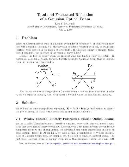
Total and Frustrated Reflection of a Gaussian Optical Beam 1 ...

1 Problem
Total and Frustrated Reflection
of a Gaussian Optical Beam
Kirk T. McDonald
Joseph Henry Laboratories, Princeton University, Princeton, NJ 08544
(July 7, 2009)
When an electromagnetic wave in a medium with index of refraction n 1 encounters an interface
with a region of index n 2

y-polarization in a medium with permittivity ɛ and permeability μ has fields
E x ≈ 0,
E y ≈ E 0 e −ρ2 /(1+z 2 /z0 2)
√ e i{kz[1+z 0ρ 2 /k(z 2 +z0 2)]−ωt−tan−1 (z/z 0 )} , (1)
1+z 2 /z0
2
E z ≈ − 2iy e −i tan−1 z/z 0
E
kw0y
2 y √ ,
1+z 2 /z0
2
B x = − n c E y, B y =0, B z = 2ix n
kw0x
2
where c is the speed of light in vacuum,
c E y
k 0 = ω c , k = nk 0, n = c √ √
ɛμ, ρ =
e −i tan−1 z/z 0
√
1+z 2 /z 2 0
√ x2
w 2 0x
, (2)
+ y2
, (3)
w0y
2
w 0j for j = x or y is the characteristic radius of the beam at its waist (focus), θ 0j is the
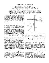
diffraction angle and z 0 is the Rayleigh range, as shown in the figure below, which are related
by
θ 0j = w 0j
z 0
,
1
= 1 + 1
z 0 kw0x
2 kw0y
2
(
z 0 = kw2 0
2 = 2
kθ 2 0
)
if w 0x = w 0y = w 0 . (4)
Near the focus (ρ < ∼ 1, |z|

equations provided w 0j ≪ z 0 , i.e., θ 0j ≪ 1. This is the case in the present problem, where
we wish to explore the behavior of very weakly focused optical beams.
The flow of energy in this elliptical beam is described by the (real) Poynting vector,
S =
ReE × ReB
μ
√ (
ɛ
=
μ E2 0 e−2ρ2
− 2x sin[2(kz − ωt)], − 2y sin[2(kz − ωt)], cos 2 (kz − ωt)
kw0x
2 kw0y
2
(7)
The time-average flow of energy is, of course, only in the direction of propagation of the
wave. In addition, there is an oscillatory transverse flow of energy. 3
2.2 Reflection and Refraction at a Single Interface
The classic formalism for plane waves is reviewed in Appendix B.
We first consider the refraction of a weakly focused Gaussian beam at a single interface
between linear, isotropic media of indices n 1 = c √ ɛ 1 μ 1 and n 2 = c √ ɛ 2 μ 2 , using notation
as shown in the figure below. For simplicity, we restrict our attention to the case that the
electric field is perpendicular to the plane of incidence (i.e., tothex-z plane).
)
.
The incident, reflected and transmitted beams each have the Gaussian form (5)-(6), with
respect to axes (x i ,y i ,z i ), (x r ,y r ,z r )and(x t ,y t ,z t ), where the z-axes are in the directions of
propagation of the various beams.
The transformation between the axes (x i ,y i ,z i ) of the incident beam and the laboratory
axes (x, y, z) is
and
x i =cosθ 1 x − sin θ 1 z, y i = y, z i =sinθ 1 x +cosθ 1 z, (8)
ρ 2 i = x2 i
+ y2 i
wix
2 wiy
2
= cos2 θ 1 x 2 − sin 2θ 1 xz +sin 2 θ 1 z 2
w 2 ix
+ y2
, (9)
wiy
2
where θ 1 is the angle between the axis of the incident beam and the z-axis, and we assume
that axis of the incident beam passes through the origin. The components of a vector A
with respect to the laboratory frame are related to those with respect to axes (x i ,y i ,z i )by
A x =cosθ 1 A xi +sinθ 1 A zi , A y = A yi , A z = − sin θ 1 A xi +cosθ 1 A zi . (10)
3 Near its waist, a Gaussian beam is similar to a wave inside a conducting wave guide, which latter case
also exhibits steady longitudinal, and oscillatory transverse, flow of energy [2].
3

Combining eqs. (5)-(10), the components of the incident beam in the laboratory frame are
E ix = −i sin θ 1 y
z 0
E iy , (11)
E iy = E 0i e −ρ2 i e
i(n 1 sin θ 1 k 0 x+n 1 cos θ 1 k 0 z−ωt) , (12)
E iz = −i cos θ 1 y
E iy , (13)
z 0
B ix = n [
]
1
cos θ 1 x − sin θ 1 z
cos θ 1 − i sin θ 1 E iy , (14)
c
z 0
B iy = 0 (15)
B iz = n [
]
1
cos θ 1 x − sin θ 1 z
sin θ 1 + i cos θ 1 E iy . (16)
c
z 0
Similarly, the reflected beam is related by
x r = − cos θ 1 x − sin θ 1 z, y r = y, z r = − sin θ 1 x − cos θ 1 z, (17)
ρ 2 r = x2 r
+ y2 r
wrx
2 wrx
2
= cos2 θ 1 x 2 +sin2θ 1 xz +sin 2 θ 1 z 2
w 2 rx
+ y2
,, (18)
wrx
2
A x = − cos θ 1 A xi +sinθ 1 A zi , A y = A yi , A z = − sin θ 1 A xi − cos θ 1 A zi , (19)
E rx = −i sin θ 1 y
E ry ,
z 0
(20)
E ry = E 0r e −ρ2 r e
i(n 1 sin θ 1 k 0 x−n 1 cos θ 1 k 0 z−ωt) , (21)
E rz = i cos θ 1 y
E iy ,
z 0
(22)
B rx = n [
]
1
cos θ 1 x +sinθ 1 z
− cos θ 1 + i sin θ 1 E ry ,
c
z 0
(23)
B ry = 0 (24)
B rz = n [
]
1
cos θ 1 x +sinθ 1 z
sin θ 1 + i cos θ 1 E ry ,
c
z 0
(25)
where we have assumed that the reflected beam also makes angle θ 1 with respect to the
z-axis, and that the axis of the reflected beam passes through the origin.
Likewise, the transmitted beam is related by
x t =cosθ 2 x − sin θ 2 z, y t = y, z t =sinθ 2 x +cosθ 2 z, (26)
ρ 2 t = x2 t
+ y2 t
wtx
2 wty
2
= cos2 θ 2 x 2 − sin 2θ 2 xz +sin 2 θ 2 z 2
w 2 tx
+ y2
, (27)
wty
2
A x =cosθ 2 A xt +sinθ 2 A zt , A y = A yt , A z = − sin θ 2 A xt +cosθ 2 A zt , (28)
4

E tx = −i sin θ 2 y
E ty ,
z 0t
(29)
E ty = E 0t e −ρ2 t e
i(n 2 sin θ 2 k 0 x+n 2 cos θ 2 k 0 z−ωt) , (30)
E tz = −i cos θ 2 y
E ty ,
z 0t
(31)
B tx = n 2
c
B tz = n 2
c
[
]
cos θ 2 x − sin θ 2 z
cos θ 2 − i sin θ 2 E ty ,
z 0t
(32)
B ty = 0 (33)
[
]
cos θ 2 x − sin θ 2 z
sin θ 2 + i cos θ 2 E ty .
z 0t
(34)
The boundary conditions at the interface z =0arethatE ⊥ , D z = ɛE z , B z and H ⊥ =
B ⊥ /μ are continuous. Thus, continuity of E y
E 0i e −ρ2 i e
i(n 1 sin θ 1 k 0 x−ωt) + E 0r e −ρ2 r e
i(n 1 sin θ 1 k 0 x−ωt) = E 0t e −ρ2 t e
i(n 2 sin θ 2 k 0 x−ωt) , (35)
for all x and y, which confirms the assumption that θ r = θ i = θ i , verifies Snell’s law,
tells us that beam waists are related by
n 1 sin θ 1 = n 2 sin θ 2 , (36)
w ix = w rx = cos θ 1
w tx ,
cos θ 2
w iy = w ry = w ty , (37)
and that the wave amplitudes are related by
Similarly, the continuity of H x = B x /μ tells us that
E 0i + E 0r = E 0t . (38)
n 1 cos θ 1
μ 1
(E 0i − E 0r )= n 2 cos θ 2
μ 2
E 0t . (39)
Combining eqs. (38) and (39) we obtain the usual Fresnel relations 4 for polarization perpendicular
to the plane of incidence,
E 0r
= n 1 cos θ 1 − μ 1
n
μ 2 cos θ 2
2
E 0i n 1 cos θ 1 + μ ,
1
n
μ 2 cos θ 2 2
E 0t
E 0i
=
2n 1 cos θ 1
n 1 cos θ 1 + μ . (40)
1
n
μ 2 cos θ 2 2
Furthermore, the continuity of E x (or D z = ɛE z ) tells us that the Rayleigh ranges are related
by
z 0i = z 0r = sin θ 1
z 0t = n 2
z 0t . (41)
sin θ 2 n 1
Equation (41) is not quite consistent with eqs. (4) and (37).
4 See Appendix B
5

In the remainder of the body of this note we suppose that μ 1 = μ 2 = μ 0 , where the
latter is the permeability of the vacuum. We also suppose that the incident Gaussian beam
is circularly symmetric, and write the incident waist as w ix = w iy = w 1 . It follows that
the reflected Gaussian beam is also circularly symmetric with the same waist w 1 . The
incident and reflected beams have Rayleigh range z 0i = k 1 w1/2 2 =n 1 k 0 w1/2, 2 while that of
the transmitted beam is z 0t = n 1 z 0i /n 2 .
2.3 Total Reflection at a Single Interface
The phenomenon of total reflection at an interface between optically denser and lighter media
wasdiscussedbyNewtoninProposition96ofhisPrincipia [3], and in further detail in his
Opticks [4]. Newton’s model was that particles of light are attracted by the denser medium,
and so follow curved rays that result in an offset between the incident and reflected path, as
shown in the figure on the left below (from the Principia).
Newton’s prediction was largely forgotten after the success of the wave theory of light in
the early 1800’s, but was occasionally discussed in the first half of the 20 th century [5, 6, 7, 8].
Then, in 1947 Goos and Hänchen [9] provided experimental evidence for what is now called
the Goos-Hänchen shift, d, illustrated in the figure on the above right.
Total reflection occurs when the indices of the two media obey n 1 >n 2 and the angle of
incidence, θ 1 , is large enough that sin θ 2 =(n 1 /n 2 )sinθ 1 > 1. In this case,
cos θ 2 =
√
√
n 2
1 − sin 2 1 sin 2 θ 1 − n 2 2
θ 2 = i
, (42)
n 2
is purely imaginary. As a consequence, the amplitudes (40) of the reflected and transmitted
waves include a phase shift relative to that of the incident wave, while
|E 0r | = |E 0i | , and
|E 0t | 2
|E 0i | 2 = 4n2 1 cos 2 θ 1
. (43)
n 2 1 − n 2 2
The quantity ρ 2 t
of eq. (27) can now be written
√
ρ 2 t = (n2 2 − n 2 1 sin 2 θ 1 ) x 2 − 2in 1 sin θ 1 n 2 1 sin 2 θ 1 − n 2 2 xz + n 2 1 sin 2 θ 1 z 2
+ y2
. (44)
n 2 2wtx
2 wty
2
6

Hence, matching of this form to that of ρ 2 i at z = 0 requires that
ρ 2 t = cos2 θ 1 x 2
w 2 1
+ y2
w 2 1
− n2 1 sin2 θ 1 cos 2 θ 1 z 2
(n 2 1 sin 2 θ 1 − n 2 2)w 2 1
+2i n 1 sin θ 1 cos 2 θ 1 xz
√
, (45)
n 2 1 sin 2 θ 1 − n 2 2 w1
2
recalling eq. (9). The factor e −Re(ρ2 t ) is constant on surfaces that are elliptical hyperboloids
of 1 sheet about the z-axis, with asymptotic opening angle θ txz in the x-z plane given by
tan θ txz =
n 1 sin θ 1
√
> 1. (46)
n 2 1 sin 2 θ 1 − n 2 2
This potentially dramatic behavior is, however, masked by the damping of the transmitted
wave in z, as follows from the factor
e i(n 2 sin θ 2 k 0 x+n 2 cos θ 2 k 0 z−ωt) = e −√ n 2 1 sin2 θ 1 −n 2 2 k 0z e i(n 1 sin θ 1 k 0 x−ωt) . (47)
The time-average flow of energy in medium 2 is given by
〈S〉 = Re(E t × B ⋆ t )
= 1 Re [E ty Btz ⋆ 2μ 0 2μ ˆx +(E tzBtx ⋆ − E tx Btz) ⋆ ŷ − E ty Btx ⋆ ẑ]
0
⎡ ⎛ √
⎞
= n 2 |E 0t | 2
e −2Re(ρ2 t ) e −2√ n 2 1 sin2 θ 1
n
−n 2 2 k 0z ⎣sin θ 2
⎝1 2 1 sin 2 θ 1 − n 2 2 z
−
⎠ ˆx
2μ 0 c
z 0t
√
− sin θ ⎤
2 n 2 1 sin 2 θ 1 − n 2 2 x
ẑ. ⎦
z 0t
≈ |E 0t| 2
√
2μ 0 c e−2Re(ρ2 t ) e −2 n 2 1 sin2 θ 1 −n 2 2 k0z sin θ 1
(n 1ˆx − n √
)
2x
n 2 1 sin 2 θ 1 − n 2 2 ẑ , (48)
z 0i
noting that z 0t = n 1 z 0i /n 2 .
Energy flows in the +x direction in medium 2, but this flow is significant only near the
origin because of exponential damping factors. Furthermore, energy flows in the +z direction
for x>0andinthe−z direction for x>0. That is, energy flows in curves in medium 2, as
qualitatively predicted by Newton. Lines of 〈S〉 that enter medium 2 from medium 1 at −x
return to medium 1 at +x.
In particular, the flow of energy between media 1 and 2 across the plane z =0isdescribed
by
〈S z 〉 2→1
= − |E 0i| 2 4n 2 1n 2 cos 2 θ 1 sin θ 1
√n 2 1 sin 2 θ 1 − n 2 2 x
e −2(cos2 θ 1 x 2 +y 2 )/w
2μ 0 c n 2 1 − n 2 1 2 , (49)
2
z 0i
recalling eq. (43). This energy adds to that in the nominal reflected wave at z =0forx>0,
〈S z 〉 r
= − 1
2μ 0
Re (E ry (z =0)B ⋆ rx(z =0))=− |E 0i| 2
2μ 0 c n 1 cos θ 1 e −2(cos2 θ 1 x 2 +y 2 )/w 2 1 , (50)
7

and subtracts from that for x

To deduce all components of the electric and magnetic fields of a Gaussian beam from a
single scalar wave function, we follow the suggestion of Davis [27] and seek solutions for a
vector potential A that has only a single Cartesian component (such that (∇ 2 A) j = ∇ 2 A j
[28]). We work in the Lorenz gauge (and SI units), so that the electric scalar potential Φ is
related to the vector potential A by
∇ · A = − n2
c 2 ∂Φ
∂t = ω
in2 c 2
Φ=ik2 Φ. (54)
ω
The vector potential can therefore have a nonzero divergence, which permits solutions having
only a single component.
Of course, the electric and magnetic fields can be deduced from the potentials via
E = −∇Φ − ∂A
∂t = i ω ∇(∇ · A)+iωA, (55)
k2 using the Lorenz condition (54), and
B = ∇ × A. (56)
The vector potential satisfies the free-space (Helmholtz) wave equation,
∇ 2 A − n2 ∂ 2 A
c 2 ∂t 2 =(∇2 + k 2 )A =0. (57)
We seek a solution in which the vector potential is described by a single Cartesian component
A j that propagates in the +z direction with the form
A j (r) =ψ(r)e i(kz−ωt) . (58)
Inserting trial solution (58) into the wave equation (57) we find that
∇ 2 ψ +2ik ∂ψ =0. (59)
∂z
In the usual analysis, one now assumes that the beam is cylindrically symmetric about
the z axis and can be described in terms of three geometric parameters the diffraction angle
θ 0 ,thewaistw 0 , and the depth of focus (Rayleigh range) z 0 , which are related by
θ 0 = w 0
= 2 , and z 0 = kw2 0
z 0 kw 0 2 = 2
kθ 2 . (60)
0
9

Here, we consider the possibility that the beam has an elliptical cross section, with major
and minor axes along the x and y axes. The waist and diffraction angle are different in the
x-z and y-z planes, but the Rayleigh range is in common:
θ 0x = w 0x
, and θ 0y = w 0y
. (61)
z 0 z 0
We now convert to the scaled coordinates
ξ =
x
w 0x
, υ = y
w 0y
, ρ 2 = ξ 2 + υ 2 , and ς = z z 0
. (62)
Changing variables and noting relations (61), the wave equation (59) takes the form
1
w 2 0x
∂ 2 ψ
∂ξ 2 + 1 ∂ 2 ψ
w0y
2 ∂υ + 1 ∂ 2 ψ
2 z0
2 ∂ς + 2ik ∂ψ
2 z 0 ∂ς
=0. (63)
The paraxial approximation is that the term in the relatively small quantity 1/z 2 0 is neglected,
and the resulting paraxial wave equation is
1
w 2 0x
∂ 2 ψ
∂ξ 2 + 1 ∂ 2 ψ
w0y
2 ∂υ + 2ik ∂ψ
2 z 0 ∂ς
≈ 0. (64)
An “educated guess” is that the transverse behavior of the wave function ψ has a Gaussian
form, but with a width that varies with z. Also, the amplitude of the wave far from its waist
should vary as 1/z. In the scaled coordinates ρ and ς a trial solution is
ψ = h(ς)e −f(ς)ρ2 , (65)
where the possibly complex functions f and h are defined to obey f(0) = 1 = h(0). Since
the transverse coordinate ξ and υ are scaled by the waists w 0x and w 0y ,weseethatRe(f) =
w 2 0j /w2 j (ς) wherew j(ς) is the beam width in coordinate j = x or y at position ς. Fromthe
geometric parameters (62) we see w j (ς) ≈ θ 0j z = w 0j ς for large ς. Hence, we expect that
Re(f) ≈ 1/ς 2 for large ς. Also, we expect the amplitude h to obey |h| ≈1/ς for large ς.
Plugging the trial solution (65) into the paraxial wave equation (64) we find that
( 1
− fh
w 2 0x
+ 1 ) ( ) ξ
2
+2f 2 h + υ2
+ ik (h ′ − f ′ hρ 2 ) ≈ 0, (66)
w0y
2 w0x
2 w0y
2 z 0
where a ′ indicates differentiation with respect to ς. We can define the Rayleigh range z 0
and the waists w 0x and w 0y to be related by
so eq. (66) can be rewritten as
− fh+ ih ′ + ρ 2 h
(
1
w 2 0x
+ 1
)
= k , (67)
w0y
2 z 0
[ ( ) ]
2z0 ξ
2
+ υ2
f 2 − if ′ ≈ 0. (68)
kρ 2 w0x
2 w0y
2
10

If w 0x = w 0y , eq. (68) reduces to the form
− fh+ ih ′ + ρ 2 h(f 2 − if ′ ) ≈ 0, (69)
recalling eq. (60). The key approximation of this note is that eq. (68) can be written
as eq. (69) even when w 0x ≠ w 0y .
Accepting this approximation, we see that for eq. (69) to be true at all values of ρ implies
that
f ′
f = −i, and h ′
= −i. (70)
2 fh
Thus, f = h is a solution, despite the different physical origin of these two functions as the
transverse width and amplitude of the wave. We integrate the first of eq. (70) to obtain
1
= C + iς. (71)
f
Our definition f(0) = 1 determines that C =1. Thatis,
f = 1
1+iς = 1 − iς
1+ς 2 = e−i tan−1 ς
√
1+ς
2 . (72)
Note that Re(f) = 1/(1 + ς 2 ) = w 2 0j/w 2 j (ς), while |f| = 1/ √ 1+ς 2 , so that f = h is
consistent with the asymptotic expectations discussed above. The longitudinal dependences
of the widths of the Gaussian beam are now seen to be
The lowest-order wave function is
w j (ς) =w 0j
√
1+ς
2
. (73)
ψ 0 = fe −fρ2 = e−i tan−1 ς
√
1+ς
2 e−ρ2 /(1+ς 2) e iςρ2 /(1+ς 2) . (74)
The factor e −i tan−1 ς in ψ 0 is the so-called Gouy phase shift [29], which changes from 0 to π/2
as z varies from 0 to ∞, with the most rapid change near the z 0 . For large z the phase
factor e iςρ2 /(1+ς 2) can be written as e i(z 0/z)(x 2 /w 2 0x +y2 /w 2 0y ) ≈ e ikr2 ⊥ /(2z) , recalling eqs. (62) and
(67). When this is combined with the traveling wave factor e i(kz−ωt) we have
e i[kz(1+r2 ⊥ /2z2)−ωt] ≈ e i(kr−ωt) , (75)
√
where r = z 2 + r⊥. 2 Thus, the wave function ψ 0 is a modulated spherical wave for large z,
but is a modulated plane wave near its waist.
To obtain the electric and magnetic fields of a Gaussian beam that is polarized in the y
direction we take the vector potential to be
Then,
A x =0, A y = E 0
iω ψ 0e i(kz−ωt) = E 0
iω fe−fρ2 e i(kz−ωt) , A z =0. (76)
∇ · A = − 2fy A
w0y
2 y . (77)
11

and the electric field follows from eq. (55) as
E x ≈ 0, E y ≈ E 0 fe −fρ2 e i(kz−ωt) , E z ≈− 2iyf E
kw0y
2 y , (78)
where we neglect terms of order 1/z 2 0. Similarly, the magnetic field follows from eq. (56) as
B x = − √ ɛμE y = − n c E y, B y =0, B z = 2ixf n
kw0x
2 c E y. (79)
B
Fresnel Relations for Plane Waves
For reference we present a derivation of the well-known Fresnel relations for reflection and
refraction of a plane wave at a planar interface.
The geometry and notation are again as shown in the figure below, with the plane of
incidence being the x-z plane.
The incident, reflected and transmitted waves can be written
E i = E 0i e i(k ixx+k iz z−ωt) , E r = E 0r e i(krxx+krzz−ωt) , E t = E 0t e i(ktxx+ktzz−ωt) , (80)
B i = k i
ω ×E 0i e i(k ixx+k iz z−ωt) ,
B r = k r
ω ×E 0r e i(krxx+krzz−ωt) ,
B t = k t
ω ×E 0t e i(ktxx+ktzz−ωt) ,
(81)
where we have used the plane-wave Maxwell equation ik × E = ∇ × E = −∂B/∂t = iωB,
and we note that the wave equation ∇ 2 E = ∂ 2 E/∂t 2 requires that
k 2 i = k 2 ix + k 2 iz = n2 1 ω2
c 2 , k 2 r = k 2 rx + k 2 rz = n2 1 ω2
c 2 , k 2 t = k 2 tx + k 2 tz = n2 2 ω2
c 2 , (82)
so that
k i = k r = n 1
k t . (83)
n 2
Continuity of the tangential component of E at the interface requires that the argument of
the exponential factors all be equal there, and hence
k ix = k rx = k tx , (84)
12

θ i = θ r = θ 1 , k rz = −k iz , (85)
and
n 1 sin θ 1 = n 2 sin θ 2 (= n 2 sin θ t ). (86)
Then, the continuity of the x- andy-components of E = μωH×k/k 2 at the interface implies
H 0iy − H 0ry = μ 2 n 2 1 k tz
H
μ 1 n 2 0ty = μ 2 n 1 cos θ 2
H 0ty , and E 0iy + E 0ry = E 0ty , (87)
2 k iz μ 1 n 2 cos θ 1
noting that E x ∝ μk z H y /n 2 . Similarly, continuity of the tangential component of H =
k × E/μω at the interface implies
E 0iy − E 0ry = μ 1
μ 2
k tz
k iz
E 0ty = μ 1
μ 2
n 2 cos θ 2
n 1 cos θ 1
E 0ty , and H 0iy + H 0ry = H 0ty . (88)
noting that H x ∝ k z H y /μ. Combining eqs. (87) and (88) we find
E 0ry
= n 1 cos θ 1 − μ 1
n
μ 2 cos θ 2
2
E 0iy n 1 cos θ 1 + μ ,
1
n
μ 2 cos θ 2 2
E 0ty
E 0iy
=
2n 1 cos θ 1
n 1 cos θ 1 + μ , (89)
1
n
μ 2 cos θ 2 2
H 0ry
= n 2 cos θ 1 − μ 2
n
μ 1 cos θ 2
1
H 0ty 2n 2 cos θ 1
H 0iy n 2 cos θ 1 + μ , =
2
n
μ 1 cos θ 2 H 0iy n 2 cos θ 1 + μ . (90)
2
n
1 μ 1 cos θ 2 1
For the special case of the electric field polarized perpendicular to the plane of incidence, H
has no y-component, and we write
E 0r⊥
= n 1 cos θ 1 − μ 1
n
μ 2 cos θ 2
2
E 0t⊥ 2n 1 cos θ 1
E 0i⊥ n 1 cos θ 1 + μ , =
1
n
μ 2 cos θ 2 E 0i⊥ n 1 cos θ 1 + μ , (91)
1
n
2 μ 2 cos θ 2 2
Similarly, for the special case of the electric field polarized parallel to the plane of incidence,
E has no y-component, and for each of the three waves, H y ∝ nE ‖ /μ, sowecanwrite
E 0r‖
E 0i‖
=
μ 1
n
μ 2 cos θ 1 − n 1 cos θ 2
2
μ 1
,
n
μ 2 cos θ 1 + n 1 cos θ 2 2
E 0t‖
E 0i‖
=
2n 1 cos θ 1
μ 1
, (92)
n
μ 2 cos θ 1 + n 1 cos θ 2 2
As usual, we note that the case of internal reflection when sin θ 2 =(n 1 /n 2 )sinθ 1 > 1can
be accommodated in the above formalism by writing
cos θ 2 =
√
1 − sin 2 θ 2 =
√
n 2 2 − n 2 1 sin 2 θ 1
n 2
= i
√
n 2 1 sin 2 θ 1 − n 2 2
n 2
. (93)
In this case, we also write
√
n 2 1 sin 2 θ 1 − n 2 2
k tz = ik 0 , (94)
n 2
such that the transmitted wave is damped in z according to
(√ )
e iktzz = e − n 2
1 sin 2 θ 1 −n 2 2 /n 2 k 0 z
. (95)
13

References
[1] K.T. McDonald, Gaussian Laser Beams with Radial Polarization (Mar. 14, 2000),
http://puhep1.princeton.edu/~mcdonald/examples/axicon.pdf
[2] M. Moriconi and K.T. McDonald, Energy Flow in a Waveguide below Cutoff (Mar. 14,
2000), http://puhep1.princeton.edu/~mcdonald/examples/cutoff.pdf
[3] I. Newton, Principa, Vol. 1 (London, 1726; reprint of Cajori’s English translation, U.
Calif. Press, 1962), Proposition 96.
[4] I. Newton, Opticks, 4th ed. (London, 1730; Dover, New York, 1952).
Book Two, Part 1, Observation 1: “Compressing two Prisms hard together that their
sides (which by chance were a very little convex) might somewhere touch one another:
I found the place in which they touched to become absolutely transparent, as if they
had there been one continued piece of Glass. For when the Light fell so obliquely on the
Air, which in other places was between them, as to be all reflected; it seemed in that
place of contact to be wholly transmitted, .....”
Book Three, Part 1, Question 29: “Are not the Rays of Light very small Bodies emitted
from shining Substances? For such Bodies will pass through uniform Media in Right
Lines without bending into the Shadow, which is the Nature of Rays of Light. ..... The
Rays of Light in going out of Glass into a Vacuum, are bent towards the Glass; and
if they fall too obliquely on the Vacuum, ther are bent backwards into the Glass, and
totally reflected; and this Reflexion cannot be ascribed to the Resistance of an absolute
Vacuum, but must be caused the the Power of the Glass attracting the Rays at their
going out of it into the Vacuum, and bringing them back.”
[5] S. Boguslawski, Das Feld des Poyntingschen Vektors bei der Interferenz von zwei ebenen
Lichtwellen in einem absorbierenden Medium, Phys.Z.13, 393 (1912),
http://puhep1.princeton.edu/~mcdonald/examples/optics/boguslawski_pz_13_393_12.pdf
[6]A.Wiegrefe,Neue Lichtströmungen bei Totalreflexion. Beiträge zur Diskussion des
Poyntingschen Satzes, Ann. Phys. 45, 30 (1914),
http://puhep1.princeton.edu/~mcdonald/examples/optics/wiegrefe_ap_45_30_14.pdf
Neue Lichtströmungen bei Totalreflexion. Beiträge zur Kenntnis des Poyntingschen Vektors,
Ann. Phys. 50, 277 (1914),
http://puhep1.princeton.edu/~mcdonald/examples/optics/wiegrefe_ap_50_277_16.pdf
H. Rose and A. Wiegrefe, Versuche über die Sichtbarmachung von Lichtströmungen
durch die Einfallsebene im isotropen Medium bei Totalreflexion, Ann. Phys. 50, 281
(1916), http://puhep1.princeton.edu/~mcdonald/examples/optics/rose_ap_50_281_16.pdf
[7] J. Picht, Beitrag zur Theorie der Totalreflexion, Ann. Phys. 3, 433 (1929),
http://puhep1.princeton.edu/~mcdonald/examples/optics/picht_ap_3_433_29.pdf
Die Energieströmung bei der Totalreflexion, Phys.Z.30, 905 (1929),
http://puhep1.princeton.edu/~mcdonald/examples/optics/picht_pz_30_905_29.pdf
14

[8] C. Schaefer and R. Pich, Ein Beitrag zur Theorie der Totalreflexion, Ann. Phys. 30,
245 (1937),
http://puhep1.princeton.edu/~mcdonald/examples/optics/schaefer_ap_30_245_37.pdf
[9] F. Goos and H. (Lindberg-)Hänchen, Ein neuer und fundamentaler Versuch zur Totalreflexion,
Ann. Phys. 1, 333 (1947),
http://puhep1.princeton.edu/~mcdonald/examples/optics/goos_ap_1_333_47.pdf
Neumessung des Strahlversetzungseffektes bei Totalreflexion, Ann. Phys. 5, 251 (1949),
http://puhep1.princeton.edu/~mcdonald/examples/optics/goos_ap_5_251_49.pdf
[10] K. Artmann, Zur Seitenversetzung des totalreflektierten Lichtstrahles, Ann. Phys. 2, 87
(1948), http://puhep1.princeton.edu/~mcdonald/examples/optics/artmann_ap_2_87_48.pdf
[11] C. von Fragstein Berechnung der Seitenversetzung des totalreflektierten Strahles, Ann.
Phys. 4, 18 (1949),
http://puhep1.princeton.edu/~mcdonald/examples/optics/vonfragstein_ap_4_18_49.pdf
[12] H. Wolter, Untersuchengen zur Strahlversetzung bei Totalreflexiondes Lichtes mit der
Methode der Minimumstrahlkennzeichnung, Z.Natur.5a, 143 (1950),
http://puhep1.princeton.edu/~mcdonald/examples/optics/wolter_zn_5a_143_50.pdf
[13] R.H. Renard, Total Reflection: A New Evaluation of the Goos-Hänchen Shift, J.Opt.
Soc. Am. 54, 1190 (1964),
http://puhep1.princeton.edu/~mcdonald/examples/optics/renard_josa_54_1190_64.pdf
[14] H.K.V. Lotsch, Reflection and and Refraction of Light at a Plane Interface, J.Opt.Soc.
Am. 58, 551 (1968),
http://puhep1.princeton.edu/~mcdonald/examples/optics/lotsch_josa_58_551_68.pdf
Beam Displacement at Total Reflection: The Goos-Hänchen Effect, Optik,32, 116, 189,
300, 563 (1970),
http://puhep1.princeton.edu/~mcdonald/examples/optics/lotsch_optik_32_116_70.pdf
[15] C. Imbert, Calculation and Experimental Proof of the Transverse Shift Induced by Total
Internal Reflection of a Circularly Polarized Light Beam, Phys.Rev.D5, 787 (1972),
http://puhep1.princeton.edu/~mcdonald/examples/optics/imbert_prd_5_787_72.pdf
[16] B.R. Horowitz and T. Tamir, Lateral Displacement of a Light Beam at a Dielectric
Interface, J.Opt.Soc.Am.61, 586 (1971),
http://puhep1.princeton.edu/~mcdonald/examples/optics/horowitz_josa_61_586_71.pdf
[17] L. de Broglie and J.P Vigier, Photon Mass and New Experimental Results on Longitudinal
Displacements of Laser Beams near Total Reflection, Phys. Rev. Lett. 28, 1001
(1972),
http://puhep1.princeton.edu/~mcdonald/examples/optics/debroglie_prl_28_1001_72.pdf
[18] K.W Chiu and J.J. Quinn, On the Goos-Hänchen Effect. A Simple Example of a Time
Delay Scattering Process, Am.J.Phys.40, 1847 (1972),
http://puhep1.princeton.edu/~mcdonald/examples/optics/chiu_ajp_40_1847_72.pdf
15

[19] J.W. Ra, H.L. Bertoni and L.B. Felsen, Reflection and Transmission of Beams at a
Dielectric Interface, SIAM J. Appl. Math. 24, 396 (1973),
http://puhep1.princeton.edu/~mcdonald/examples/optics/ra_siamjam_24_396_73.pdf
[20] Y.M. Antar and W.B. Boerner, Reflection and Refraction of a Gaussian Beam at a
Planar Dielectric Interface, Ant. Prop. Soc. Int. Symp. 12, 105 (1974),
http://puhep1.princeton.edu/~mcdonald/examples/optics/antar_apsim_12_105_74.pdf
[21] S. Zhu, A.W. Yu, D. Hawley and R. Roy, Frustrated total internal reflection: A demonstration
and review, Am.J.Phys.54, 601 (1986),
http://puhep1.princeton.edu/~mcdonald/examples/optics/zhu_ajp_54_601_86.pdf
[22] P. Hillion, Gaussian Beam at a Dielectric Interface, J.Opt.(Paris)25, 155 (1994),
http://puhep1.princeton.edu/~mcdonald/examples/optics/hillion_jop_25_155_94.pdf
[23] D.A. Papathanassoglou and B. Vohnsen, Direct visualization of evanescent optical
waves, Am.J.Phys.71, 670 (2003),
http://puhep1.princeton.edu/~mcdonald/examples/optics/papathanassoglou_ajp_71_670_03.pdf
[24] H.G.L. Schwefel et al., Direct experimental observation of the single reflection optical
Goos-Hänchen shift, Opt. Lett. 33, 794 (2008),
http://puhep1.princeton.edu/~mcdonald/examples/optics/schwefel_ol_33_794_08.pdf
[25] J.C. Bose, On the Influence of the Thickness of Air-space on Total Reflection of Electric
Radiation, Proc. Roy. Soc. London 62, 300 (1897),
http://puhep1.princeton.edu/~mcdonald/examples/optics/bose_prsl_62_300_97.pdf
[26] E.E. Hall, The Penetration of Totally Reflected Light into the Rarer Medium, Phys.
Rev. 15, 73 (1902),
http://puhep1.princeton.edu/~mcdonald/examples/optics/hall_pr_15_73_02.pdf
[27] L.W. Davis, Theory of electromagnetic beams, Phys.Rev.A19, 1177-1179 (1979),
http://puhep1.princeton.edu/~mcdonald/examples/optics/davis_pra_19_1177_79.pdf
[28] P.M. Morse and H. Feshbach, Methods of Theoretical Physics, Part I (McGraw-Hill,
New York, 1953), pp. 115-116.
[29] G. Gouy, Sur une propreite nouvelle des ondes lumineuases, Compt. Rendue Acad. Sci.
(Paris) 110, 1251 (1890); Sur la propagation anomele des ondes, ibid. 111, 33 (1890),
http://puhep1.princeton.edu/~mcdonald/examples/optics/gouy_cr_110_1251_90.pdf
http://puhep1.princeton.edu/~mcdonald/examples/optics/gouy_cr_111_33_90.pdf
16