Polarization Dependence of Emissivity - Physics Department ...

Polarization Dependence of Emissivity
David J. Strozzi
Department of Physics, Massachusetts Institute of Technology, Cambridge, MA 02139
Kirk T. McDonald
Joseph Henry Laboratories, Princeton University, Princeton, NJ 08544
(April 3, 2000)
1 Problem
Deduce the emissive power of radiation of frequency ν into vacuum at angle θ to the normal
to the surface of a good conductor at temperature T , for polarization both parallel and
perpendicular to the plane of emission.
2 Solution
The solution is adapted from ref. [1] (see also [2]), and finds application in the calibration of
the polarization dependence of detectors for cosmic microwave background radiation [3, 4].
Recall Kirchhoff’s law of heat radiation (as clarified by Planck [5]) that
P ν
A ν
= K(ν, T ) = hν3 /c 2
e hν/kT − 1 , (1)
where P ν is the emissive power per unit area per unit frequency interval (emissivity) and
∣ E
A ν = 1 − R = 1 −
0r ∣∣∣
2
∣
E 0i
is the absorption coefficient (0 ≤ A ν ≤ 1), c is the speed of light, h is Plank’s constant and
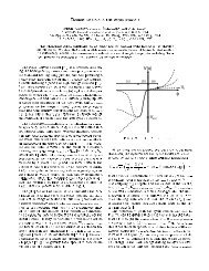
k is Boltzmann’s constant. Also recall the Fresnel equations of reflection that
(2)
E 0r
E 0i
∣ ∣∣∣⊥
= sin(θ t − θ i )
sin(θ t + θ i ) ,
E 0r
E 0i
∣ ∣∣∣‖
= tan(θ t − θ i )
tan(θ t + θ i ) , (3)
where i, r, and t label the incident, reflected, and transmitted waves, respectively.
The solution is based on the fact that eq. (1) holds separately for each polarization of
the emitted radiation, and is also independent of the angle of the radiation. This result is
implicit in Planck’s derivation [5] of Kirchhoff’s law of radiation, and is stated explicitly in
[6]. That law describes the thermodynamic equilibrium of radiation emitted and absorbed
throughout a volume. The emissivity P v and the absorption coefficient A ν can depend on
the polarization of the radiation and on the angle of the radiation, but the definitions of
polarization parallel and perpendicular to a plane of emission, and of angle relative to the
normal to a surface element, are local, while the energy conservation relation P ν = A ν K(ν, T )
is global. A “ray” of radiation whose polarization can be described as parallel to the plane of
emission is, in general, a mixture of parallel and perpendicular polarization from the point
of view of the absorption process. Similarly, the angles of emission and absorption of a ray
1

are different in general. Thus, the concepts of parallel and perpendicular polarization and
of the angle of the radiation are not well defined after integrating over the entire volume.
Thermodynamic equilibrium can exist only if a single spectral intensity function K(ν, T )
holds independent of polarization and of angle.
All that remains is to evaluate the reflection coefficients R ⊥ and R ‖ for the two polarizations
at a vacuum-metal interface. These are well known [1, 2, 7], but we derive them for
completeness.
To use the Fresnel equations (3), we need expressions for sin θ t and cos θ t . The boundary
condition that the phase of the wave be continuous across the vacuum-metal interface leads,
as is well known, to the general form of Snell’s law:
k i sin θ i = k t sin θ t , (4)
where k = 2π/λ is the wave number. Then,
cos θ t = √ 1 − k2 i
sin 2 θ
kt
2 i . (5)
To determine the relation between wave numbers k i and k t in vacuum and in the conductor,
we consider a plane wave of angular frequency ω = 2πν and complex wave vector
k,
E = E 0 e i(k t·r−ωt) , (6)
which propagates in a conducting medium with dielectric constant ɛ, permeability µ, and
conductivity σ. The wave equation for the electric field in such a medium is (in Gaussian
units)
∇ 2 E − ɛµ ∂ 2 E
c 2 ∂t = 4πµσ ∂E
2 c 2 ∂t , (7)
where c is the speed of light. We find the dispersion relation for the wave vector k t on
inserting eq. (6) in eq. (7):
kt 2 = ɛµ ω2
c + i4πσµω . (8)
2 c 2
For a good conductor, the second term of eq. (8) is much larger than the first, so we write
where
k t ≈
√ 2πσµω
c
d =
(1 + i) = 1 + i
d
=
2
d(1 − i) , (9)
c
√ 2πσµω
≪ λ (10)
is the frequency-dependent skin depth. Of course, on setting ɛ = 1 = µ and σ = 0 we obtain
expressions that hold in vacuum, where k i = ω/c.
We see that for a good conductor |k t | ≫ k i , so according to eq. (5) we may take cos θ t ≈ 1
to first order of accuracy in the small ratio d/λ. Then the first of the Fresnel equations
becomes
∣
E 0r ∣∣∣⊥
= cos θ i sin θ t / sin θ i − 1
E 0i cos θ i sin θ t / sin θ i + 1 = (k i/k t ) cos θ i − 1
(k i /k t ) cos θ i + 1 ≈ (πd/λ)(1 − i) cos θ i − 1
(πd/λ)(1 − i) cos θ i + 1 , (11)
2

and the reflection coefficient is approximated by
∣ E
R ⊥ =
0r ∣∣∣
2
∣
E 0i
For the other polarization, we see that
so that
⊥
≈ 1 − 4πd
λ cos θ i = 1 − 2 cos θ i
√ ν
σ . (12)
E 0r
E 0i
∣ ∣∣∣‖
= E 0r
E 0i
∣ ∣∣∣⊥ cos(θ i + θ t )
cos(θ i − θ t ) ≈ E 0r
E 0i
∣ ∣∣∣⊥ cos θ i − (πd/λ)(1 − i) sin 2 θ i
cos θ i + (πd/λ)(1 − i) sin 2 θ i
, (13)
R ‖ ≈ R ⊥
(
1 − 4πd
λ
sin 2 )
θ i
≈ 1 −
cos θ i
4πd = 1 − 2 √ ν
λ cos θ i cos θ i σ . (14)
An expression for R ‖ valid to second order in d/λ has been given in ref. [7]. For θ i near 90 ◦ ,
R ⊥ ≈ 1, but eq. (14) for R ‖ is not accurate. Writing θ i = π/2 − ϑ i with ϑ i ≪ 1, eq. (13)
becomes
∣
E 0r ∣∣∣‖
≈ ϑ i − (πd/λ)(1 − i)
E 0i ϑ i + (πd/λ)(1 − i) , (15)
For θ i = π/2, R ‖ = 1, and R ‖,min = (5 − √ 2)/(5 + √ 2) = 0.58 for ϑ i = 2 √ 2πd/λ.
Finally, combining eqs. (1), (2), (12) and (14) we have
and
P ν⊥ ≈
4πd cos θ
λ 3
hν
e hν/kT − 1 , P ν‖ ≈ 4πd
λ 3 cos θ
hν
e hν/kT − 1 , (16)
P ν⊥
P ν‖
= cos 2 θ (17)
for the emissivities at angle θ such that cos θ ≫ d/λ.
The conductivity σ that appears in eq. (16) can be taken as the dc conductivity so long
as the wavelength exceeds 10 µm [1]. If in addition hν ≪ kT , then eq. (16) can be written
P ν⊥ ≈
4πd kT cos θ
λ 3 , P ν‖ ≈
4πd kT
λ 3 cos θ , (18)
in terms of the skin depth d.
We would like to thank Matt Hedman, Chris Herzog and Suzanne Staggs for conversations
about this problem.
3 References
[1] M. Born and E. Wolf, Principles of Optics, 7th ed., (Cambridge U. Press, Cambridge,
1999), sec. 14.2.
[2] L.D. Landau and E.M. Lifshitz, The Electrodynamics of Continuous Media (Pergamon
Press, Oxford, 1960), sec. 67.
3

[3] E.J. Wollack, A measurement of the degree scale cosmic background radiation anisotropy
at 27.5, 30.5, and 33.5 GHz, Ph.D. dissertation (Princeton University, 1994), Appendix
C.1.1.
[4] C. Herzog, Calibration of a Microwave Telescope, Princeton U. Generals Expt. (Oct.
26, 1999).
[5] M. Planck, The Theory of Heat Radiation (Dover Publications, New York, 1991),
chap. II, especially sec. 28.
[6] F. Reif, Fundamentals of statistical and thermal physics (McGraw-Hill, New York, 1965),
sec. 9.14.
[7] J.A. Stratton, Electromagnetic Theory (McGraw-Hill, New York, 1941), sec. 9.9.
4