Vector calculus in curvilinear coordinates Goals: Coordinate ...
Vector calculus in curvilinear coordinates Goals: Coordinate ...
Vector calculus in curvilinear coordinates Goals: Coordinate ...

You also want an ePaper? Increase the reach of your titles
YUMPU automatically turns print PDFs into web optimized ePapers that Google loves.
<strong>Vector</strong> <strong>calculus</strong> <strong>in</strong> curvil<strong>in</strong>ear coord<strong>in</strong>ates<br />
D. Jaksch<br />
<strong>Goals</strong>:<br />
• Understand the difference between coord<strong>in</strong>ates and vector components<br />
• Understand the implications of basis vectors <strong>in</strong> curvil<strong>in</strong>ear coord<strong>in</strong>ates not be<strong>in</strong>g constant<br />
• Learn how to use curvil<strong>in</strong>ear coord<strong>in</strong>ate systems <strong>in</strong> vector <strong>calculus</strong><br />
Coord<strong>in</strong>ate systems and vector fields<br />
Coord<strong>in</strong>ate systems<br />
A po<strong>in</strong>t <strong>in</strong> coord<strong>in</strong>ate space r is often represented as r = (x, y, z) T with x, y, and z the distances along the<br />
three coord<strong>in</strong>ate axes. We can equally <strong>in</strong>troduce cyl<strong>in</strong>drical polar coord<strong>in</strong>ates which we will use here as the<br />
prime example for curvil<strong>in</strong>ear coord<strong>in</strong>ate systems. They are def<strong>in</strong>ed through the relations<br />
x = ρ cos(ϕ), y = ρ s<strong>in</strong>(ϕ), and z = z.<br />
The po<strong>in</strong>t <strong>in</strong> space is now written as r = (ρ cos(ϕ), ρ s<strong>in</strong>(ϕ), z) T<br />
that they give the distances along the three coord<strong>in</strong>ate axes.<br />
where the mean<strong>in</strong>g of the components is still<br />
<strong>Vector</strong> fields<br />
A vector field assigns a vector to each po<strong>in</strong>t r and is usually denoted as F(r) or simply F. The vector field<br />
is often def<strong>in</strong>ed through components F i (r) which are the projections of the vector onto the three coord<strong>in</strong>ate<br />
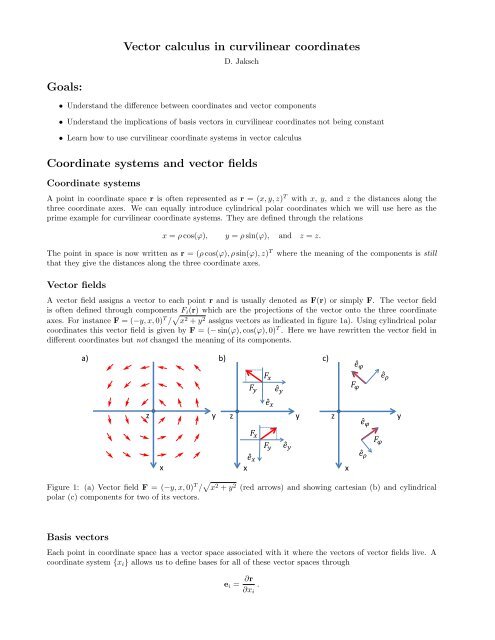
axes. For <strong>in</strong>stance F = (−y, x, 0) T / √ x 2 + y 2 assigns vectors as <strong>in</strong>dicated <strong>in</strong> figure 1a). Us<strong>in</strong>g cyl<strong>in</strong>drical polar<br />
coord<strong>in</strong>ates this vector field is given by F = (− s<strong>in</strong>(ϕ), cos(ϕ), 0) T . Here we have rewritten the vector field <strong>in</strong><br />
different coord<strong>in</strong>ates but not changed the mean<strong>in</strong>g of its components.<br />
a) b) c)<br />
F x<br />
F y<br />
êy<br />
êφ<br />
F φ<br />
êρ<br />
êx<br />
z<br />
y<br />
z<br />
y<br />
z<br />
êφ<br />
y<br />
x<br />
F x<br />
êx<br />
x<br />
F y<br />
êy<br />
x<br />
êρ<br />
F φ<br />
Figure 1: (a) <strong>Vector</strong> field F = (−y, x, 0) T / √ x 2 + y 2 (red arrows) and show<strong>in</strong>g cartesian (b) and cyl<strong>in</strong>drical<br />
polar (c) components for two of its vectors.<br />
Basis vectors<br />
Each po<strong>in</strong>t <strong>in</strong> coord<strong>in</strong>ate space has a vector space associated with it where the vectors of vector fields live. A<br />
coord<strong>in</strong>ate system {x i } allows us to def<strong>in</strong>e bases for all of these vector spaces through<br />
e i = ∂r<br />
∂x i<br />
.
For cartesian coord<strong>in</strong>ates the normalized basis vectors are ê x = î, ê y = ĵ, and ê z = ˆk po<strong>in</strong>t<strong>in</strong>g along the three<br />
coord<strong>in</strong>ate axes. They are orthogonal, normalized and constant, i.e. their direction does not change with the<br />
po<strong>in</strong>t r 1 .<br />
Next we calculate basis vectors for a curvil<strong>in</strong>ear coord<strong>in</strong>ate systems us<strong>in</strong>g aga<strong>in</strong> cyl<strong>in</strong>drical polar coord<strong>in</strong>ates.<br />
They are given by<br />
ê ρ = ∂r<br />
∂ρ = cos(ϕ)ê x + s<strong>in</strong>(ϕ)ê y ,<br />
ê ϕ = 1 ∂r<br />
ρ ∂ϕ = − s<strong>in</strong>(ϕ)ê x + cos(ϕ)ê y , and ê z = ê z .<br />
The 1/ρ <strong>in</strong> the def<strong>in</strong>ition of ê ϕ is required for the vector to be properly normalized to 1. These basis vectors<br />
are mutually orthogonal and normalized. However, they are not constant, their direction changes with position.<br />
By <strong>in</strong>vert<strong>in</strong>g this set of l<strong>in</strong>ear equations for the basis vectors we f<strong>in</strong>d<br />
ê x = cos(ϕ)ê ρ − s<strong>in</strong>(ϕ)ê ϕ , ê y = s<strong>in</strong>(ϕ)ê ρ + cos(ϕ)ê ϕ , and ê z = ê z .<br />
We can now write a vector field F(r) = (F x (r), F y (r), F z (r)) T c ≡ F x (r)ê x + F y (r)ê y + F z (r)ê z <strong>in</strong> new<br />
components us<strong>in</strong>g the above relations between the basis vectors for different coord<strong>in</strong>ate systems. This is still<br />
the same vector field but now written as F(r) = (F ρ (r), F ϕ (r), F z (r)) T p ≡ F ρ (r)ê ρ + F ϕ (r)ê ϕ + F z (r)ê z . The<br />
new components are projections on the basis vectors ê ρ , ê ϕ , and ê z . We use <strong>in</strong>dices c and p to make explicit<br />
which components are used. In detail, the change of components is carried out by<br />
F =<br />
⎛<br />
⎝<br />
F x<br />
F y<br />
⎞<br />
⎠ = F x ê x + F y ê y + F z ê z = F x [cos(ϕ)ê ρ − s<strong>in</strong>(ϕ)ê ϕ ]<br />
F z c<br />
⎛<br />
F x cos(ϕ) + F y s<strong>in</strong>(ϕ)<br />
⎞<br />
+F y [s<strong>in</strong>(ϕ)ê ρ + cos(ϕ)ê ϕ ] + F z ê z = ⎝ −F x s<strong>in</strong>(ϕ) + F y cos(ϕ) ⎠<br />
F z<br />
Cartesian and cyl<strong>in</strong>drical polar components for the vector field F = (− s<strong>in</strong>(ϕ), cos(ϕ), 0) T c = (0, 1, 0) T p are shown<br />
<strong>in</strong> figures 1b) and 1c) respectively. Produce a similar figure for the vector field F = r = (x, y, z) T c = (ρ, 0, z) T p .<br />
The most commonly used coord<strong>in</strong>ate systems produce orthogonal right handed bases. This means that scalar<br />
and vector products between the basis vectors obey the familiar relations ê i · ê j = δ ij and ê i × ê j = ê k ɛ ijk ,<br />
where δ ij is the Kronecker delta and ɛ ijk the totally antisymmetric tensor. For cyl<strong>in</strong>drical polar coord<strong>in</strong>ates<br />
(ρ, ϕ, z) we explicitly have<br />
ê ρ · ê ρ = ê ϕ · ê ϕ = ê z · ê z = 1 and ê ρ · ê ϕ = ê ϕ · ê z = ê z · ê ρ = 0 ,<br />
ê ρ × ê ρ = ê ϕ × ê ϕ = ê z × ê z = 0, ê ρ × ê ϕ = ê z , ê ϕ × ê z = ê ρ and ê z × ê ρ = ê ϕ ,<br />
<strong>Vector</strong> Calculus<br />
Partial derivatives<br />
The partial derivatives with respect to the coord<strong>in</strong>ates are found us<strong>in</strong>g the cha<strong>in</strong> rule 2<br />
∂ ρ = cos(ϕ)∂ x + s<strong>in</strong>(ϕ)∂ y , ∂ ϕ = −ρ s<strong>in</strong>(ϕ)∂ x + ρ cos(ϕ)∂ y , and ∂ z = ∂ z ,<br />
p<br />
and<br />
∂ x = cos(ϕ)∂ ρ − s<strong>in</strong>(ϕ) ∂ ϕ ,<br />
ρ<br />
∂ y = s<strong>in</strong>(ϕ)∂ ρ + cos(ϕ) ∂ ϕ , and ∂ z = ∂ z .<br />
ρ<br />
∇-operator<br />
We now rewrite the ∇-operator by us<strong>in</strong>g these relations<br />
⎛ ⎞<br />
⎛<br />
∂ x<br />
∇ = ⎝ ∂ y<br />
⎠ = ê x ∂ x + ê y ∂ y + ê z ∂ z = ê ρ ∂ ρ + êϕ<br />
ρ ∂ ϕ + ê z ∂ z = ⎝<br />
∂ z<br />
c<br />
∂ ρ<br />
1<br />
ρ ∂ ϕ<br />
∂ z<br />
⎞<br />
⎠<br />
p<br />
1 This might seem obvious but needs to be revisited <strong>in</strong> relativity and has far reach<strong>in</strong>g consequences for the physical nature of<br />
space.<br />
2 The calculation is identical to work<strong>in</strong>g out the basis vectors but replac<strong>in</strong>g ∂r/∂i → ∂ i . The partial derivatives can thus directly<br />
be read off from the relations between the basis vectors.
Gradient<br />
The gradient of a scalar field U <strong>in</strong> cyl<strong>in</strong>drical polar coord<strong>in</strong>ates is now given by<br />
⎛<br />
gradU = ∇U = ⎝<br />
∂U<br />
∂ρ<br />
1 ∂U<br />
ρ ∂ϕ<br />
∂U<br />
∂z<br />
⎞<br />
⎠<br />
p<br />
= ê ρ ∂ ρ U + êϕ<br />
ρ ∂ ϕU + ê z ∂ z U .<br />
The expression for the ∇-operator <strong>in</strong> cyl<strong>in</strong>drical polar components is thus <strong>in</strong>directly given on the data-sheet 3 .<br />
There you will f<strong>in</strong>d an expression for ∇U and the del-operator is found by simply leav<strong>in</strong>g out U <strong>in</strong> this expression.<br />
Divergence<br />
When work<strong>in</strong>g out the divergence we need to properly take <strong>in</strong>to account that the basis vectors are not constant<br />
<strong>in</strong> general curvil<strong>in</strong>ear coord<strong>in</strong>ates. For cyl<strong>in</strong>drical polar coord<strong>in</strong>ates we have two nonzero derivatives<br />
∂ ϕ ê ϕ = − cos(ϕ)ê x − s<strong>in</strong>(ϕ)ê y = −ê ρ and ∂ ϕ ê ρ = − s<strong>in</strong>(ϕ)ê x + cos(ϕ)ê y = ê ϕ .<br />
The divergence will thus <strong>in</strong> general not be given by ∇ · F(r) = ∑ i ∂ iF i (r) which is only true for an orthogonal<br />
coord<strong>in</strong>ate system whose basis vectors are constant <strong>in</strong> space. Us<strong>in</strong>g the product rule we f<strong>in</strong>d<br />
∇ · F = [ê ρ ∂ ρ + êϕ<br />
ρ ∂ ϕ + ê z ∂ z ] · [F ρ ê ρ + F ϕ ê ϕ + F z ê z ] = ∂ ρ F ρ + êϕ<br />
ρ · [∂ ϕ(F ρ ê ρ ) + ∂ ϕ (F ϕ ê ϕ )] + ∂ z F z<br />
Rotation<br />
= ∂ ρ F ρ + êϕ<br />
ρ · [ê ρ∂ ϕ F ρ + F ρ ê ϕ + ê ϕ ∂ ϕ F ϕ − ê ρ F ϕ ] + ∂ z F z = ∂ ρ(ρF ρ )<br />
+ ∂ ϕF ϕ<br />
+ ∂ z F z .<br />
ρ ρ<br />
The calculation is similar to work<strong>in</strong>g out the divergence<br />
∇ × F = [ê ρ ∂ ρ + êϕ<br />
ρ ∂ ϕ + ê z ∂ z ] × [F ρ ê ρ + F ϕ ê ϕ + F z ê z ] = ê ρ × [ê ϕ ∂ ρ F ϕ + ê z ∂ ρ F z ] +<br />
ê ϕ<br />
ρ × [ê ρ∂ ϕ F ρ − ê ρ F ϕ + ê z ∂ ϕ F z ] + ê z × [ê ρ ∂ z F ρ + ê ϕ ∂ z F ϕ ]<br />
= ê ρ<br />
[<br />
∂ϕ F z<br />
ρ<br />
]<br />
[<br />
∂ρ (ρF ϕ )<br />
− ∂ z F ϕ + ê ϕ [−∂ ρ F z + ∂ z F ρ ] + ê z − ∂ ]<br />
ϕF ρ<br />
.<br />
ρ ρ<br />
Laplace operator<br />
We obta<strong>in</strong> the Laplace operator by replac<strong>in</strong>g F → ∇ <strong>in</strong> the expression for the divergence<br />
∆ = ∇ · ∇ = 1 ρ ∂ ρ(ρ∂ ρ ) + 1 ρ 2 ∂2 ϕ + ∂ 2 z .<br />
Example<br />
A velocity field describ<strong>in</strong>g a vortex is given by u = Aê ϕ /ρ with A a constant. Its divergence and rotation are<br />
given by<br />
[<br />
]<br />
∇ · u = ê ρ ∂ ρ + êϕ<br />
ρ ∂ ϕ + ê z ∂ z · Aê [<br />
]<br />
ϕ<br />
= 0 , ∇ × u = ê ρ ∂ ρ + êϕ<br />
ρ<br />
ρ ∂ ϕ + ê z ∂ z × Aê ϕ<br />
= A ρ ρ 2 (ê z − ê z ) = 0 .<br />
The acceleration of a parcel of fluid is given by (this term appears <strong>in</strong> the Navier Stokes equation)<br />
(u · ∇)u = A ρ 2 ∂ Aê ϕ<br />
ϕ = − A ρ ρ 3 êρ .<br />
Work out these expressions us<strong>in</strong>g cartesian components.<br />
3 Also spherical polar coord<strong>in</strong>ates can be found on the data sheet.
Summary<br />
Cyl<strong>in</strong>drical polar coord<strong>in</strong>ates (ρ, ϕ, z)<br />
• Relation to cartesian coord<strong>in</strong>ates (care is required to obta<strong>in</strong> ϕ <strong>in</strong> the correct quadrant)<br />
x = ρ cos(ϕ) , y = ρ s<strong>in</strong>(ϕ) and z = z<br />
ρ = √ x 2 + y 2 , ϕ = arctan(y/x) and z = z<br />
• Basis vectors ê ρ = ∂ ρ r, ρê ϕ = ∂ ϕ r, ê z = ∂ z r<br />
ê ρ = cos(ϕ)ê x + s<strong>in</strong>(ϕ)ê y , ê ϕ = − s<strong>in</strong>(ϕ)ê x + cos(ϕ)ê y and ê z = ê z<br />
ê x = cos(ϕ)ê ρ − s<strong>in</strong>(ϕ)ê ϕ , ê y = s<strong>in</strong>(ϕ)ê ρ + cos(ϕ)ê ϕ and ê z = ê z<br />
• Non-zero derivatives of basis vectors<br />
∂ ϕ ê ρ = ê ϕ ,<br />
∂ ϕ ê ϕ = −ê ρ<br />
• ∇-operator<br />
• Divergence<br />
• Rotation<br />
∇ × F(r) = ê ρ<br />
[<br />
∂ϕ F z<br />
ρ<br />
∇ = ê ρ ∂ ρ + êϕ<br />
ρ ∂ ϕ + ê z ∂ z<br />
∇ · F = ∂ ρ(ρF ρ )<br />
ρ<br />
+ ∂ ϕF ϕ<br />
ρ<br />
+ ∂ z F z<br />
]<br />
[<br />
∂ρ (ρF ϕ )<br />
− ∂ z F ϕ + ê ϕ [−∂ ρ F z + ∂ z F ρ ] + ê z − ∂ ]<br />
ϕF ρ<br />
ρ ρ<br />
• Laplace<br />
∆ = 1 ρ ∂ ρ(ρ∂ ρ ) + 1 ρ 2 ∂2 ϕ + ∂ 2 z<br />
Spherical polar coord<strong>in</strong>ates (r, θ, ϕ)<br />
• Relation to cartesian and cyl<strong>in</strong>drical coord<strong>in</strong>ates (care is required to obta<strong>in</strong> ϕ <strong>in</strong> the correct quadrant)<br />
x = r cos(ϕ) s<strong>in</strong>(θ) , y = r s<strong>in</strong>(ϕ) s<strong>in</strong>(θ) , z = r cos(θ) and ρ = r s<strong>in</strong>(θ)<br />
r = √ x 2 + y 2 + z 2 , ϕ = arctan(y/x) and θ = arccos(z/r) = arctan(ρ/z)<br />
• Basis vectors ê r = ∂ r r, rê θ = ∂ θ r, r s<strong>in</strong>(θ)ê ϕ = ∂ ϕ r<br />
ê r = cos(θ)ê z + s<strong>in</strong>(θ)ê ρ , ê θ = − s<strong>in</strong>(θ)ê z + cos(θ)ê ρ and ê ϕ = ê ϕ<br />
ê z = cos(θ)ê r − s<strong>in</strong>(θ)ê θ , ê ρ = s<strong>in</strong>(θ)ê r + cos(θ)ê θ and ê ϕ = ê ϕ<br />
ê x = s<strong>in</strong>(θ) cos(ϕ)ê r + cos(θ) cos(ϕ)ê θ − s<strong>in</strong>(ϕ)ê ϕ and ê y = s<strong>in</strong>(θ) s<strong>in</strong>(ϕ)ê r + cos(θ) s<strong>in</strong>(ϕ)ê θ + cos(ϕ)ê ϕ<br />
• Non-zero derivatives of basis vectors<br />
∂ θ ê r = ê θ , ∂ θ ê θ = −ê r , ∂ ϕ ê r = s<strong>in</strong>(θ)ê ϕ , ∂ ϕ ê θ = cos(θ)ê ϕ and ∂ ϕ ê ϕ = −ê ρ<br />
• ∇-operator<br />
• Divergence<br />
∇ = ê r ∂ r + êθ<br />
r ∂ θ +<br />
êϕ<br />
r s<strong>in</strong>(θ) ∂ ϕ<br />
∇ · F = ∂ r(r 2 F r )<br />
r 2 + ∂ θ(s<strong>in</strong>(θ)F θ )<br />
+ ∂ ϕF ϕ<br />
r s<strong>in</strong>(θ) r s<strong>in</strong>(θ)<br />
• Rotation<br />
∇ × F =<br />
[<br />
êr<br />
r s<strong>in</strong>(θ) [∂ θ(F ϕ s<strong>in</strong>(θ)) − ∂ ϕ F θ ] + êθ −∂ r (rF ϕ ) + ∂ ]<br />
ϕF r<br />
+ êϕ<br />
r<br />
s<strong>in</strong>(θ) r [∂ r(rF θ ) − ∂ θ F r ]<br />
• Laplace<br />
∆ = 1 r 2 ∂ r(r 2 ∂ r ) +<br />
1<br />
r 2 s<strong>in</strong>(θ) ∂ 1<br />
θ(s<strong>in</strong>(θ)∂ θ ) +<br />
r 2 s<strong>in</strong> 2 (θ) ∂2 ϕ