Class notes - MT tutorial 4 1 Commuting operators â â
Class notes - MT tutorial 4 1 Commuting operators â â
Class notes - MT tutorial 4 1 Commuting operators â â

Create successful ePaper yourself
Turn your PDF publications into a flip-book with our unique Google optimized e-Paper software.
S.R. Clark<br />
Teaching <strong>notes</strong><br />
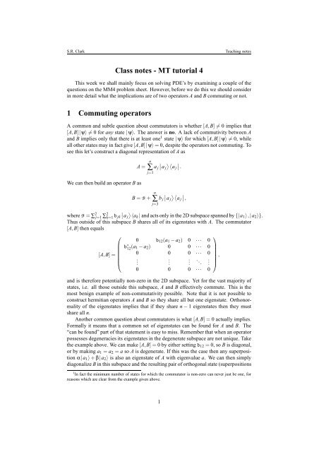
<strong>Class</strong> <strong>notes</strong> - <strong>MT</strong> <strong>tutorial</strong> 4<br />
This week we shall mainly focus on solving PDE’s by examining a couple of the<br />
questions on the MM4 problem sheet. However, before we do this we should consider<br />
in more detail what the implications are of two <strong>operators</strong> A and B commuting or not.<br />
1 <strong>Commuting</strong> <strong>operators</strong><br />
A common and subtle question about commutators is whether [A,B] ≠ 0 implies that<br />
[A,B]|ψ〉 ≠ 0 for any state |ψ〉. The answer is no. A lack of commutivity between A<br />
and B implies only that there is at least one 1 state |ψ〉 for which [A,B]|ψ〉 ≠ 0, while<br />
all other states may in fact give [A,B]|ψ〉 = 0, despite the <strong>operators</strong> not commuting. To<br />
see this let’s construct a diagonal representation of A as<br />
A =<br />
We can then build an operator B as<br />
n<br />
∑<br />
j=1<br />
B =B +<br />
a j<br />
∣ ∣aj<br />
〉〈<br />
a j<br />
∣ ∣.<br />
n<br />
∑<br />
j=3<br />
b j<br />
∣ ∣aj<br />
〉〈<br />
a j<br />
∣ ∣,<br />
whereB = ∑ 2 j=1 ∑ 2 k=1 b 〉<br />
∣<br />
jk a j 〈ak | and acts only in the 2D subspace spanned by {|a 1 〉,|a 2 〉}.<br />
Thus outside of this subspace B shares all of its eigenstates with A. The commutator<br />
[A,B] then equals<br />
⎛<br />
[A,B] =<br />
⎜<br />
⎝<br />
0 b 12 (a 1 − a 2 ) 0 ··· 0<br />
b ∗ 12 (a 1 − a 2 ) 0 0 ··· 0<br />
0 0 0 ··· 0<br />
.<br />
.<br />
.<br />
. .. . 0 0 0 ··· 0<br />
and is therefore potentially non-zero in the 2D subspace. Yet for the vast majority of<br />
states, i.e. all those outside this subspace, A and B effectively commute. This is the<br />
most benign example of non-commutativity possible. Note that it is not possible to<br />
construct hermitian <strong>operators</strong> A and B so they share all but one eigenstate. Orthonormality<br />
of the eigenstates implies that if they share n − 1 eigenstates then they must<br />
share all n.<br />
Another common question about commutators is what [A,B] = 0 actually implies.<br />
Formally it means that a common set of eigenstates can be found for A and B. The<br />
“can be found” part of that statement is easy to miss. Remember that when an operator<br />
possesses degeneracies its eigenstates in the degenerate subspace are not unique. Take<br />
the example above. We can make [A,B] = 0 by either settingb 12 = 0, so B is diagonal,<br />
or by making a 1 = a 2 = a so A is degenerate. If this was the case then any superposition<br />
α|a 1 〉+β|a 2 〉 is also an eigenstate of A with eigenvalue a. We can then simply<br />
diagonalize B in this subspace and the resulting pair of orthogonal state (superpositions<br />
1 In fact the minimum number of states for which the commutator is non-zero can never just be one, for<br />
reasons which are clear from the example given above.<br />
⎞<br />
,<br />
⎟<br />
⎠<br />
1
S.R. Clark<br />
Teaching <strong>notes</strong><br />
of |a 1 〉 and |a 2 〉) are guaranteed to be eigenstates of A while also being eigenstates of<br />
B by construction. Let’s make this concrete with an example. Take A and B to be<br />
⎛<br />
A = 1 ⎝ −1 0 5 ⎞ ⎛<br />
0 4 0 ⎠ and B = 1 ⎝ 2 5 −4 ⎞<br />
5 −7 5 ⎠.<br />
2<br />
3<br />
5 0 −1<br />
−4 5 2<br />
A short calculation will reveal that [A,B] = 0. After a slightly longer calculation we<br />
can diagonalize A and B to find eigenvalues a j = {2,2,−3} with corresponding eigenvectors<br />
⎧⎛<br />
{ ∣ 〉 ⎨ a j } = ⎝ 0 ⎞ ⎛<br />
1<br />
1 ⎠, √ ⎝ 1 ⎞ ⎛<br />
1<br />
0 ⎠, √ ⎝ 1 ⎞⎫<br />
⎬<br />
0 ⎠<br />
⎩<br />
0 2 1 2 ⎭ ,<br />
−1<br />
and eigenvalues b j = {−4,1,2} with corresponding eigenvectors<br />
⎧ ⎛<br />
{ ∣ 〉 ⎨ 1<br />
b j } = √ ⎝ −1<br />
⎞ ⎛<br />
1<br />
2 ⎠, √ ⎝ 1 ⎞ ⎛<br />
1<br />
1 ⎠, √ ⎝ 1 ⎞⎫<br />
⎬<br />
0 ⎠<br />
⎩ 6 1 3 1 2 ⎭ .<br />
−1<br />
Thus the first two eigenvectors of A are degenerate, while B is non-degenerate. Notice<br />
also that as computed above A and B share precisely their third eigenvector. What this<br />
example illustrates is that because A and B commute, and B is non-degenerate, eigenvectors<br />
of B will automatically be eigenvectors of A and are the unique choice for a<br />
common eigenbasis for the two <strong>operators</strong>. However, since A is degenerate, the converse<br />
is not true, eigenvectors of A are not necessarily eigenvectors of B. The choice made<br />
above for |a 1 〉 and |a 2 〉 is precisely an example of this since neither is an eigenvector<br />
of B, whereas a simple calculation can confirm that |b 1 〉 and |b 2 〉 are eigenvectors of<br />
A. It is simple to see that we can form |b 1 〉 and |b 2 〉 as superpositions of |a 1 〉 and |a 2 〉.<br />
2 Troublesome problems explained<br />
MM question 4.5: Find all separable solutions of Laplace’s equation ∇ 2 V = 0 in 2D<br />
polar coordinates?<br />
We start by assuming that V(r,θ,φ) = R(r)S(θ) and insert this into the equation for the<br />
Laplacian in 2D polars<br />
[<br />
∇ 2 V(r,θ) = r ∂ (<br />
r ∂ ] )+ ∂2<br />
∂r ∂r ∂θ 2 V(r,θ) = 0,<br />
which gives<br />
S(θ)r ∂ ∂r<br />
(<br />
r ∂ )R(r)+R(r) ∂2<br />
S(θ) = 0.<br />
∂r<br />
∂θ2 We then rearrange and introduce a separation constant m 2 to give<br />
(<br />
r ∂<br />
r ∂ )<br />
R(r) = m 2 ,<br />
R(r) ∂r ∂r<br />
∂ 2<br />
m 2 = − 1<br />
S(θ) ∂θ 2 S(θ).<br />
2
S.R. Clark<br />
Teaching <strong>notes</strong><br />
We can immediately solve the S(θ) equation<br />
∂ 2<br />
∂θ 2 S(θ) = −m2 S(θ), (1)<br />
to get solutions S(θ) = C m e imθ = D m e −imθ with the constraint that since θ is an angular<br />
variable satisfying 0 ≤ θ ≤ 2π, then S(θ) = S(θ+2π) we have that m must be an integer<br />
or zero. This leaves an equation for R(r) of the form<br />
r ∂ (r ∂ )<br />
∂r ∂r R(r) = m 2 R(r). (2)<br />
We first solve this equation for the case when m = 0 which is equivalent to solving<br />
∂<br />
∂r R(r) = A 0<br />
r , (3)<br />
where A 0 is a constant, yielding a solution R(r) = A 0 ln(r)+B 0 . For m ≠ 0 we solve<br />
the equation using the ansatz R(r) = r k giving k 2 = m 2 implying that k = ±m. Thus we<br />
have solutions R(r) of the form<br />
{<br />
Am r m + B m r −m m > 0<br />
R(r) =<br />
A 0 ln(r)+B 0 m = 0 . (4)<br />
Linear combinations of the separable solutions R(r)S(θ) are capable of describing the<br />
most general solution because the equation is linear and homogeneous. In the question<br />
we are given the following:<br />
(i) Given V(r = a,θ) = V 0 (1+cos(θ)), and that V is finite as r → 0, find V(r,θ) in<br />
the region r ≤ a. (ii) Given, separately, that V(r = b,θ) = 2V 0 sin 2 (θ), and V is finite<br />
as r → ∞, find V(r,θ) for r ≥ b.<br />
For (i) we see that neither ln(r) nor the r −m solutions can appear so A 0 = 0 and<br />
B m = 0 for m > 0. We can then identify that m = 1 with A 1 =<br />
a 1, C 1 = D 1 =<br />
2 1V 0 and<br />
B 0 = V 0 , so<br />
r<br />
V(r,θ) = V 0 +V 0 cos(θ), (5)<br />
a<br />
for r ≤ a. For (ii) we can similarly reject r m and ln(r) solutions so A m = 0 for all m.<br />
The boundary condition at r = b is V(r = b,θ) = 1 2 V 0(2 − e 2iθ − e −2iθ ), from which we<br />
identify B 0 = V 0 , and C 2 = D 2 = − 1 2 V 0 with B 2 = b 2 . Thus the solution is<br />
for r ≥ b.<br />
V(r,θ) = V 0 −V 0<br />
b 2<br />
cos(2θ), (6)<br />
r2 MM question 4.8: Perform a separation of variables on Laplace’s equation ∇ 2 V = 0<br />
in spherical polar coordinates?<br />
We start by assuming that V(r,θ,φ) = R(r)T(θ)P(φ) and insert this into the equation<br />
for the Laplacian in spherical polars<br />
[ ( 1 ∂<br />
∇V(r,θ,φ) =<br />
r 2 r 2 ∂ )<br />
+<br />
∂r ∂r<br />
∂ 2<br />
1<br />
r 2 sin 2 (θ) ∂φ 2 + 1 ∂<br />
r 2 sin(θ) ∂θ<br />
(<br />
sin(θ) ∂ )]<br />
V(r,θ,φ),<br />
∂θ<br />
3
S.R. Clark<br />
Teaching <strong>notes</strong><br />
which then gives<br />
[ T(θ)P(φ) ∂<br />
(r 2 ∂ )<br />
r 2 ∂r ∂r R(r) + R(r)T(θ) ∂ 2 R(r)P(φ) ∂<br />
r 2 sin 2 P(φ)+<br />
(θ) ∂φ2 r 2 sin(θ) ∂θ<br />
We now separate the equation for φ first with a separation constant of −m 2 as<br />
1<br />
P(φ) ∂φ 2 P(φ) = −m2 ,<br />
[<br />
−m 2 = − sin2 (θ) ∂<br />
(r 2 ∂ )<br />
R(r) ∂r ∂r R(r) − sin(θ)<br />
T(θ)<br />
∂ 2<br />
leaving the P(φ) equation<br />
∂<br />
∂θ<br />
(<br />
sin(θ) ∂<br />
∂θ T(θ) )]<br />
= 0.<br />
(<br />
sin(θ) ∂<br />
∂θ T(θ) )]<br />
,<br />
∂ 2<br />
∂φ 2 P(φ) = −m2 P(φ). (7)<br />
We then separate the remaining equation once more with a separation constant λ as<br />
1 ∂<br />
(r 2 ∂ )<br />
R(r) ∂r ∂r R(r) = λ,<br />
(<br />
1 ∂<br />
λ = −<br />
sin(θ) ∂ )<br />
sin(θ)T(θ) ∂θ ∂θ T(θ) + m2<br />
sin 2 (θ) ,<br />
giving the R(r) and T(θ) equations<br />
∂<br />
(r 2 ∂ )<br />
∂r ∂r R(r) = λR(r), (8)<br />
− 1 (<br />
∂<br />
sin(θ) ∂ )<br />
sin(θ) ∂θ ∂θ T(θ) + m2<br />
sin 2 T(θ) = λT(θ). (9)<br />
(θ)<br />
We are now in a position to answer following sub-questions:<br />
(i) Why is m an integer or zero, (ii) Verify that for m = 0 the function T(θ) = cos(θ)<br />
is a solution for a certain value of λ, and find that value, (iii) Find solutions for R(r)<br />
corresponding to the particular value of λ determined in (ii), and (iv) What is the most<br />
general solution for V(r,θ,φ) having this dependence?<br />
For (i) we see that P(φ) = e imφ is a solution and since φ is an angular variable<br />
satisfying 0 ≤ φ ≤ 2π, then P(φ) = P(φ+2π) which immediately implies that m must<br />
be integer or zero. For (ii) we can set m = 0 and substitute T(θ) = cos(θ) into Eq. (9)<br />
and identify λ = 2. For (iii) we insert λ = 2 into Eq. (8) and find solutions by trying<br />
the ansatz R(r) = r m . This gives m(m + 1)r m = λr m , and has solutions R(r) = r and<br />
R(r) = 1 . Finally for (iv) the most general solution with this θ and φ dependence is<br />
r 2 V(r,θ,φ) = cos(θ)<br />
[Ar+ B ]<br />
r 2 , (10)<br />
where A and B are constants. Using this solution we can answer the final part of the<br />
question:<br />
An uncharged conducting sphere of radius a is placed at the origin in an initially uniform<br />
electrostatic field (0,0,E). Show that it behaves an electric dipole.<br />
4
S.R. Clark<br />
Teaching <strong>notes</strong><br />
The potential V(r,θ) satisfies the boundary condition V(r = a,θ) = 0 for all θ on<br />
r = a, since it is a conductor. At very large distances from the sphere the field must<br />
essentially be the same as if it was absent entirely, giving a boundary condition V(r →<br />
∞,θ) = −Ez = −Er cos(θ). We can now use these boundary conditions to determine<br />
the two constants A and B: firstly V(r,θ) = −Er cos(θ) at r → ∞ implies that A = −E<br />
while V(r,θ) = 0 at r = a implies B = Ea 3 giving<br />
]<br />
V(r,θ) = −E cos(θ)<br />
[r − a3<br />
r 2 . (11)<br />
Thus V(r,θ) behaves like an electric dipole as the deviation from the potential from a<br />
uniform field −Ez is ∝ cos(θ)<br />
r 2 .<br />
MM question 4.9: The temperature T(x,t) of a one-dimensional bar, whose sides are<br />
perfectly insulated, obeys the heat flow equation<br />
∂<br />
∂2<br />
T(x,t) = κ T(x,t), (12)<br />
∂t ∂x2 where κ is a positive constant. The bar extends from x = 0 to x = L and is perfectly<br />
insulated at x = L. At times t < 0 the temperature is 0 ◦ C throughout the bar and at<br />
t = 0 the uninsulated end at x = 0 is placed in contact with a heat bath at 100 ◦ C.<br />
Determine a solution for the temperature of the bar at subsequent times and estimate<br />
the time taken for the average temperature of the bar to reach 90 ◦ C if L = 1m and<br />
κ = 0.001m 2 s −1 .<br />
We start by performing separation of variables of the form T(x,t) = F(t)X(x) with a<br />
separation constant −q 2 as<br />
giving the F(t) and X(x) equations<br />
1 ∂<br />
κF(t) ∂t F(t) = −q2 ,<br />
−q 2 =<br />
∂ 2<br />
1<br />
X(x) ∂x 2 X(x),<br />
∂<br />
∂t F(t) = −κq2 F(t),<br />
∂ 2<br />
∂x 2 X(x) = −q2 X(x).<br />
These equations have solutions of the form F(t) = e −κq2t and X(x) = e iqx , and clearly<br />
our choice of separation constant was made to ensure decay in time and oscillatory<br />
solutions in space, as intuition expects. In principle q could be complex, however since<br />
T(x,t) must be real we try q being real. This gives a general solution of the form<br />
T(x,t) = T 0 +C 0 x+ ∑ e −κq2t [A q sin(qx)+B q cos(qx)], (13)<br />
q>0<br />
where A q and B q are constants, while C 0 and T 0 are constants accounting for a possible<br />
q = 0 term. When t → ∞ then we know the temperature must be in thermal equilibrium<br />
with the heat bath with a temperature of 100 ◦ C throughout. This implies that T 0 =<br />
5
S.R. Clark<br />
Teaching <strong>notes</strong><br />
100 ◦ C. At x = 0 we have that T(0,t) = T 0 for all t > 0 which gives B q = 0. The perfect<br />
insulation at x = L means that there is no heat flow at the boundary so temperature<br />
gradient must vanish there as<br />
∂<br />
∂x T(x,t) ∣<br />
∣∣∣x=L<br />
= 0. (14)<br />
This implies that C 0 = 0 and −∑ q>0 qe −κq2t A q cos(qL) = 0 for all q so<br />
q n = π L (n+ 1 2<br />
), (15)<br />
with the index n an integer. The general solution for T(x,t) is then of the form<br />
T(x,t) = T 0 +<br />
∞<br />
∑<br />
n=0<br />
e −κq2t A n sin(q n x). (16)<br />
Finally, we have the boundary condition that at t = 0 we have T(0 < x < L,0) = 0 ◦ C.<br />
To use this to fix the coefficients A n we employ the orthonormality relation<br />
Z<br />
2 L<br />
sin(q n x)sin(q m x)dx = δ nm , (17)<br />
L 0<br />
since we can multiply through by sin(q n x) and integrate to get<br />
A n + 2T 0<br />
L<br />
Z L<br />
0<br />
sin(q n x)dx = A n + 2T 0<br />
q n L . (18)<br />
Putting this together we get the full solution for T(x,t) as<br />
∞<br />
( ) [ ( )<br />
T(x,t)<br />
100 = 1 − 4 (2n+1)πx (2n+1)π 2<br />
∑<br />
n=0<br />
(2n+1)π sin exp −κ<br />
t]<br />
. (19)<br />
2L<br />
2L<br />
We can now compute the average temperature of the bar 〈T(t)〉 as<br />
〈T(t)〉 = 1 L<br />
Z L<br />
0<br />
T(x,t)dx = T 0 −<br />
∞<br />
∑<br />
n=0<br />
2T 0<br />
q 2 n L2 e−κq2nt . (20)<br />
An estimate for the time required to heat the bar to 90 ◦ C can be made by keeping only<br />
the slowest decaying term in the summation q 0 = π<br />
2L<br />
which gives<br />
T 0 − 〈T(t)〉<br />
≤ 8 ( −κπ 2 )<br />
T 0 π 2 exp t<br />
4L 2 . (21)<br />
Thus we have an estimate t c = − 4L2 ln( π2<br />
κπ 2 80<br />
) ≈ 14 minutes.<br />
6