C. Usha Devi, R. S. Bharat Chandran, R. M. Vasu and A.K. ... - Physics

More documents

Recommendations

Info

Devi et al.: Mechanical property assessment of tissue-mimicking phantoms… modulation of the detected intensity or amplitude autocorrelation. 11 The depth of modulation is influenced by the local absorption coefficient of the medium insonified by the US beam. This result added an extra dimension to DOT imaging, allowing the possibility of spatial resolution improvement of absorption coefficient images by discarding all detected diffuse photons except those tagged by ultrasound. The flurry of activity in this direction saw the arrival of a new branch of DOT known as ultrasound-assisted optical tomography UAOT. 12–14 However, it was only recently that the influence of the local microrheological properties of the turbid medium on the UAOT measurement which is the depth of modulation of the intensity or amplitude autocorrelation has been investigated. Since the US beam subjects the scattering centers in the object to an extra periodic stress, in addition to the thermal stress, the modulation in the detected photon correlation is also related to the amplitude of vibration of the scattering centers. This amplitude, in turn, is influenced by the local visco-elastic properties. 15 In Ref. 15 it is shown that the depth of modulation in the autocorrelation is influenced by the amplitude of vibration u of the scattering centers and n the modulation of the refractive index because of insonification, in addition to the local absorption coefficient. In fact, the phase modulation suffered by light owing to n and u results in modulation of the detected intensity, providing a carrier whose amplitude is influenced by the local absorption coefficient in the region of insonification through multiplication. In Ref. 15 it is pointed out that if the UAOT read-out is to be employed for a quantitatively accurate recovery of either the optical or elastic properties of the object, the influence each of these has on the modulation depth has to be first estimated and accounted for. Out of these, the contribution of absorption can be independently estimated, by reconstructing the absorption coefficient distribution using the established DOT reconstruction algorithm on the measured intensity autocorrelation g 2 at =0, which is the same as the intensity data. The remaining contributions are from refractive index fluctuations n and the path length fluctuations u. We show in this work that the displacement introduced by the focused US beam in the region of insonification is along the axis of the US transducer. Therefore, assuming that tissue-like material has a scattering anisotropy g of 0.9 light scattering is forward directed, the path length modulation and its variation with elastic property picked up by light launched perpendicular to the US transducer axis is small compared to that picked up by light along the transducer axis. This variation is negligible for storage modulus above 50 kPa, which is slightly above the normal value of healthy breast tissue. 16 In addition, it is shown through simulations and experiments that the modulation in g 2 for light launched along and perpendicular to the US axis approach the same constant pedestal value as the storage modulus of the material is increased beyond 80 kPa. This value of storage modulus is dependent also on the power input through the US transducer. When the radiation force from the US force increases, significant displacement components still influence the g 2 modulation depth, much beyond the 80-kPa limit of the present experiments. This implies that for such large stiffness, the displacement of tissue particles introduced by US radiation force is negligibly small, and the contribution to modulation in g 2 is entirely because of n j j , where j is the average undisturbed scattering path length in the insonified region. This pedestal value to which the g 2 modulation approaches is the same for both axial and transverse light interrogation, in spite of the fact that the length of interaction for these two cases is not the same. The axial length of the US focal region is approximately four times its width at the center see Sec. 2. But the path length modulation that can be picked up in diffusing wave spectroscopy has a maximum value of , the wavelength of the interrogating light. 17 For this reason the g 2 modulation depth in the two directions of interrogations approaches the same value when the storage modulus is large. This residual value, which is insensitive to storage modulus variations for storage modulus beyond 50 kPa for transverse illumination and 80 kPa for axial illumination, is the contribution from n. This means that for other values of storage modulus, wherein the g 2 modulation has contribution from both displacement and n, the contribution from n can be subtracted out, and the modulation arising entirely out of displacement of scattering centers can be ascertained. This paves the way for retrieving the displacement components induced by the US force from measurement of g 2 modulation depth, which can be used for quantitative reconstruction of the storage modulus. As a consequence of the previous observation, we suggest through this study that the absorption coefficient map obtained from g 2 modulation depth in an UAOT experiment is least likely to be affected by storage modulus variations which certainly accompanies malignant regions along with absorption coefficient increase when the interrogation light is perpendicular to the US transducer axis and the insonification is from a focused US transducer. In this case, the contribution to g 2 modulation depth from displacement is significantly less and varies very little with storage modulus. The summary of the work reported here is as follows. In Sec. 2 the force distribution in the focal region of the US transducer is calculated by solving the Westervelt equation 18 for the input parameters of the transducer and the acoustic properties of the phantom used in the experiments later. The force distribution is used in the forward elastography equation in Sec. 3, which is solved for the tissue-mimicking phantom, assuming it to be purely elastic. It is seen that the estimated displacement distribution is along the US transducer axis. Section 4 describes the simulation of propagation of photons through the insonified phantom. The goal of the simulation is the estimation of g 2 and its modulation. Photons are transported both along and perpendicular to the axis of the US transducer. Section 5 reports the experimental verification of the simulations on special tissue-mimicking phantoms. In this section, the results of simulation are compared with the corresponding experimental results. In Sec. 6 the results are discussed, and Sec. 7 puts forth the concluding remarks. 2 Force Distribution in the Focal Region of the Ultrasound Transducer The object, which is a slab of tissue-mimicking material, is insonified by radiation from a focusing US transducer. The tissue particles in the focal region are set in vibratory motion by the force of the US beam. In this section, our objective is Journal of Biomedical Optics 024028-2 March/April 2007 Vol. 122
Devi et al.: Mechanical property assessment of tissue-mimicking phantoms… to find the force distribution in the focal region of the transducer. This can be obtained from the oscillatory force experienced by the tissue particles, which is given by Ft = F 0 cost + . This force is proportional to pt, the time-dependent pressure at the focal region given by pt = p cost. Therefore, the force distribution can be obtained if one can calculate the pressure distribution in the focal region of the transducer. The governing equation for the propagation of acoustic pressure p, in situations where nonlinearities cannot be neglected, is the Khokhlov-Zabolotskaya-Kuznetzov KZK equation. Assuming the nonlinearity is mild, and without distinguishing thermodynamic and kinematic nonlinearities, the following equation known as the Westervelt equation approximates the KZK equation to model the propagation of p: 18 2 p − 1 2 p c 2 t 2 + 3 p c 4 t 3 + 2 p 2 c 4 2 =0, 3 t where is the sound diffusivity and is the coefficient of nonlinearity, a property of the medium. The frequencydependent absorption coefficient in terms of diffusivity can be expressed as 1 2 = 2 2c 3 . The parameter is usually expressed as =1+B/2A, where B/A is a factor related to nonlinearities in media. Usually is taken as 6.2 for breast tissue. 19 In this work, Eq. 3 is solved numerically for p in the focal region of a focusing ultrasound transducer using the procedure described by Kamakura, Ishiwata, and Matsuda. 18 For this, the Westervelt equation is first written in an oblate spheroidal coordinate system, which helps one to write it as two separate spheroidal beam equations: one valid in the focal region of the transducer, where the nonlinearities have to be invoked and the wave is assumed plane; and the other close to the source, where the wave is assumed to be spherically converging. The pressure waves, which are distorted owing to the presence of the nonlinear terms, are expanded using the Fourier series, which results in two sets of coupled nonlinear partial differential equations PDEs the two sets are for the two regions for the Fourier coefficients. These PDEs are solved numerically using the finite difference scheme. 18 The details of the US transducer used in the experiments, and borrowed herein for the simulations, are as follows. The central frequency of operation =1 MHz, focal length of the transducer d is 50 mm, and its aperture radius a is 25 mm, giving a full aperture angle of 60 deg. The tissue properties are taken to be those of the tissue-mimicking phantoms used in our experiments: average sound velocity =1545 msec −1 , sound absorption coefficient=1 dB/cm at 1 MHz, and density =1000 kg/m 3 . 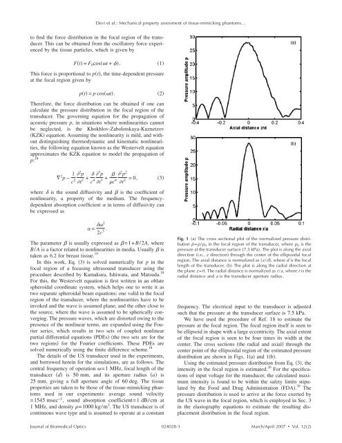The US transducer is of continuous wave type and is assumed to operate at a constant Fig. 1 a The cross sectional plot of the normalized pressure distribution p¯ =p/p 0 in the focal region of the transducer, where p 0 is the pressure at the transducer surface 7.5 kPa. The plot is along the axial direction i.e., z direction through the center of the ellipsoidal focal region. The axial distance is normalized as z/d, where d is the focal length of the transducer. b The plot is along the radial direction at the plane z=0. The radial distance is normalized as r/a, where r is the radial distance and a is the transducer aperture radius. frequency. The electrical input to the transducer is adjusted such that the pressure at the transducer surface is 7.5 kPa. We have used the procedure of Ref. 18 to estimate the pressure at the focal region. The focal region itself is seen to be ellipsoid in shape with a large eccentricity. The axial extent of the focal region is seen to be four times its width at the center. The cross sections the radial and axial through the center point of the ellipsoidal region of the estimated pressure distribution are shown in Figs. 1a and 1b. Using the estimated pressure distribution from Eq. 3, the intensity in the focal region is estimated. 20 For the specifications of input voltage for the transducer, the calculated maximum intensity is found to be within the safety limits stipulated by the Food and Drug Administration FDA. 20 The pressure distribution is used to arrive at the force exerted by the US wave in the focal region, which is employed in Sec. 3 in the elastography equations to estimate the resulting displacement distribution in the focal region. Journal of Biomedical Optics 024028-3 March/April 2007 Vol. 122
Page 1: Journal of Biomedical Optics 122, 0
Page 5 and 6: Devi et al.: Mechanical property as

C. Usha Devi, R. S. Bharat Chandran, R. M. Vasu and A.K. ... - Physics

You also want an ePaper? Increase the reach of your titles

Delete template?

Save as template?