Magnetic phase diagram of the Hubbard model in three dimensions ...
Magnetic phase diagram of the Hubbard model in three dimensions ...
Magnetic phase diagram of the Hubbard model in three dimensions ...

Create successful ePaper yourself
Turn your PDF publications into a flip-book with our unique Google optimized e-Paper software.
PHYSICAL REVIEW B<br />
VOLUME 55, NUMBER 2<br />
1 JANUARY 1997-II<br />
<strong>Magnetic</strong> <strong>phase</strong> <strong>diagram</strong> <strong>of</strong> <strong>the</strong> <strong>Hubbard</strong> <strong>model</strong> <strong>in</strong> <strong>three</strong> <strong>dimensions</strong>:<br />
The second-order local approximation<br />
A. N. Tahvildar-Zadeh<br />
Department <strong>of</strong> Physics, University <strong>of</strong> C<strong>in</strong>c<strong>in</strong>nati, C<strong>in</strong>c<strong>in</strong>nati, Ohio 45221<br />
J. K. Freericks<br />
Department <strong>of</strong> Physics, Georgetown University, Wash<strong>in</strong>gton, D.C. 20057-0995<br />
M. Jarrell<br />
Department <strong>of</strong> Physics, University <strong>of</strong> C<strong>in</strong>c<strong>in</strong>nati, C<strong>in</strong>c<strong>in</strong>nati, Ohio 45221<br />
Received 25 April 1996<br />
A local, second-order truncated approximation is applied to <strong>the</strong> <strong>Hubbard</strong> <strong>model</strong> <strong>in</strong> <strong>three</strong> <strong>dimensions</strong>.<br />
Lower<strong>in</strong>g <strong>the</strong> temperature, at half-fill<strong>in</strong>g, <strong>the</strong> paramagnetic ground state becomes unstable towards <strong>the</strong> formation<br />
<strong>of</strong> a commensurate sp<strong>in</strong>-density-wave SDW state antiferromagnetism and sufficiently far away from<br />
half-fill<strong>in</strong>g towards <strong>the</strong> formation <strong>of</strong> <strong>in</strong>commensurate SDW states. The <strong>in</strong>commensurate-order<strong>in</strong>g wave vector<br />
does not deviate much from <strong>the</strong> commensurate one, which is <strong>in</strong> accordance with <strong>the</strong> experimental data for <strong>the</strong><br />
SDW <strong>in</strong> chromium alloys. S0163-18299700402-5<br />
I. INTRODUCTION<br />
Pure Cr has a sp<strong>in</strong>-density-wave SDW ground state with<br />
an order<strong>in</strong>g wave vector which is <strong>in</strong>commensurate with <strong>the</strong><br />
underly<strong>in</strong>g lattice. 1 Add<strong>in</strong>g electrons to Cr by alloy<strong>in</strong>g with<br />
Mn makes <strong>the</strong> magnetic order commensurate with <strong>the</strong> lattice<br />
and <strong>in</strong>creases <strong>the</strong> transition temperature, whereas remov<strong>in</strong>g<br />
electrons from <strong>the</strong> system by alloy<strong>in</strong>g with V drives <strong>the</strong><br />
magnetic order to a more <strong>in</strong>commensurate one, and decreases<br />
<strong>the</strong> transition temperature, eventually to zero Fig. 5.<br />
Penn 2 found qualitatively <strong>the</strong> same behavior for <strong>the</strong> ground<br />
state <strong>of</strong> a s<strong>in</strong>gle-band <strong>Hubbard</strong> <strong>model</strong> with<strong>in</strong> a mean-field<br />
approximation. The mean-field approximation leads to <strong>the</strong><br />
usual Stoner criterion for <strong>the</strong> <strong>in</strong>stability <strong>of</strong> <strong>the</strong> paramagnetic<br />
state to <strong>the</strong> formation <strong>of</strong> a SDW state. A first-order perturbation<br />
expansion <strong>of</strong> <strong>the</strong> self-energy <strong>in</strong> terms <strong>of</strong> <strong>the</strong> <strong>in</strong>teraction<br />
parameter leads to <strong>the</strong> same criterion. In this paper we extend<br />
this approximation one step fur<strong>the</strong>r to a second-order nonself-consistent<br />
expansion for <strong>the</strong> self-energy which <strong>in</strong>cludes<br />
<strong>the</strong> lowest-order quantum fluctuations. But motivated by <strong>the</strong><br />
case for large spatial <strong>dimensions</strong>, we ignore <strong>the</strong> nonlocal<br />
site-nondiagonal elements <strong>of</strong> <strong>the</strong> self-energy. 3 In fact, <strong>in</strong>clusion<br />
<strong>of</strong> <strong>the</strong> lowest-order quantum fluctuations has been<br />
shown to have a dramatic effect on transition temperatures<br />
and <strong>phase</strong> <strong>diagram</strong>s <strong>in</strong> <strong>the</strong> large-dimensional limit, and has<br />
been shown to agree with <strong>the</strong> quantum Monte Carlo QMC<br />
data over a wide range <strong>of</strong> <strong>in</strong>teraction strengths. 4–6 Numerical<br />
evidence <strong>in</strong> this latter case has also shown that <strong>the</strong> strictly<br />
truncated perturbation expansions are more accurate than any<br />
k<strong>in</strong>d <strong>of</strong> self-consistent solutions known to us, and that <strong>the</strong><br />
<strong>in</strong>clusion <strong>of</strong> higher-order terms <strong>in</strong> <strong>the</strong> self-energy does not<br />
have any effect on <strong>the</strong> transition temperatures <strong>in</strong> <strong>the</strong> limit <strong>of</strong><br />
small <strong>in</strong>teraction strengths. 4,7<br />
The <strong>Hubbard</strong> <strong>model</strong> 8 is perhaps <strong>the</strong> simplest <strong>model</strong> which<br />
can be used to study <strong>the</strong> many-body aspects <strong>of</strong> correlated<br />
electrons on a lattice. The <strong>Hubbard</strong> Hamiltonian is written <strong>in</strong><br />
<strong>the</strong> form<br />
Ht<br />
i,j,<br />
c † i, c j, c † j, c i, U n i,↑ n i,↓ , 1<br />
i<br />
where c † i, (c i, ) represents <strong>the</strong> creation destruction operator<br />
<strong>of</strong> an electron <strong>in</strong> a Wannier state <strong>of</strong> sp<strong>in</strong> (1/2 or<br />
↑↓), on site i, and n i, c † i, c i, is <strong>the</strong> electron number operator.<br />
The first term corresponds to <strong>the</strong> k<strong>in</strong>etic energy and<br />
describes <strong>the</strong> hopp<strong>in</strong>g <strong>of</strong> electrons between nearest-neighbor<br />
sites on a lattice via an overlap <strong>in</strong>tegral t. This term gives a<br />
tight-b<strong>in</strong>d<strong>in</strong>g description <strong>of</strong> <strong>the</strong> electrons <strong>in</strong> a periodic potential<br />
form<strong>in</strong>g a s<strong>in</strong>gle energy band (k)2t i1 cosk i a for<br />
3<br />
a simple cubic lattice with lattice constant a . The second<br />
term corresponds to <strong>the</strong> Coulomb repulsion between electrons.<br />
The long-range Coulomb <strong>in</strong>teraction is assumed to be<br />
screened <strong>in</strong> <strong>the</strong> solid so that only <strong>the</strong> <strong>in</strong>teraction between two<br />
electrons on <strong>the</strong> same site is reta<strong>in</strong>ed, yield<strong>in</strong>g <strong>the</strong> additional<br />
energy <strong>of</strong> U when <strong>the</strong> lattice site is doubly occupied.<br />
The <strong>model</strong> is specified by <strong>three</strong> parameters: <strong>the</strong> strength<br />
<strong>of</strong> <strong>the</strong> electron <strong>in</strong>teraction U measured relative to t);<br />
<strong>the</strong> electron density per sp<strong>in</strong> or electron-fill<strong>in</strong>g<br />
n e (1/2N) i, c † i, c i, , where N is <strong>the</strong> number <strong>of</strong> sites <strong>in</strong><br />
<strong>the</strong> lattice; and <strong>the</strong> temperature T.<br />
In Sec. II we <strong>in</strong>troduce <strong>the</strong> formalism and <strong>the</strong> approximation<br />
that we use to form <strong>the</strong> <strong>phase</strong> <strong>diagram</strong>. In Sec. III, <strong>the</strong><br />
details <strong>of</strong> <strong>the</strong> numerical calculations are described. Section<br />
IV presents <strong>the</strong> results for <strong>the</strong> second-order approximation<br />
and compares <strong>the</strong>m to <strong>the</strong> first-order approximation and <strong>the</strong><br />
QMC results. A semiquantitative comparison is also made<br />
with <strong>the</strong> experimental data for Cr. Conclusions follow <strong>in</strong> Sec.<br />
V.<br />
II. FORMALISM<br />
For a given U and n e <strong>the</strong>re may exist more than one type<br />
<strong>of</strong> sp<strong>in</strong> order for <strong>the</strong> ground state, each be<strong>in</strong>g stable at a<br />
different temperature. Here we start from <strong>the</strong> paramagnetic<br />
0163-1829/97/552/9425/$10.00 55 942 © 1997 The American Physical Society
55 MAGNETIC PHASE DIAGRAM OF THE HUBBARD MODEL IN . . .<br />
943<br />
state and f<strong>in</strong>d a criterion for <strong>the</strong> <strong>in</strong>stability towards <strong>the</strong> formation<br />
<strong>of</strong> a SDW state. To do this we couple an external<br />
magnetic field to <strong>the</strong> system and look for s<strong>in</strong>gularities <strong>in</strong> <strong>the</strong><br />
response function magnetic susceptibility as we change <strong>the</strong><br />
<strong>model</strong> parameters. The total Hamiltonian <strong>of</strong> <strong>the</strong> system <strong>in</strong> <strong>the</strong><br />
presence <strong>of</strong> <strong>the</strong> magnetic field h i is<br />
H h H<br />
i<br />
h i S i z , 2<br />
where H is <strong>the</strong> Hamiltonian <strong>in</strong> <strong>the</strong> absence <strong>of</strong> <strong>the</strong> external<br />
field found <strong>in</strong> Eq. 1 and i is <strong>the</strong> position <strong>of</strong> <strong>the</strong> ith electron<br />
with sp<strong>in</strong> S i z n i . The spatial variation <strong>of</strong> <strong>the</strong> external<br />
field h i is chosen to probe <strong>the</strong> particular expected order<br />
for <strong>the</strong> sp<strong>in</strong>s. For example, if we want to exam<strong>in</strong>e <strong>the</strong> <strong>in</strong>stability<br />
towards antiferromagnetism, we choose h i to be <strong>of</strong> <strong>the</strong><br />
same magnitude everywhere but <strong>of</strong> <strong>the</strong> opposite sign on <strong>the</strong><br />
two sublattices <strong>of</strong> <strong>the</strong> bipartite lattice.<br />
The static response <strong>of</strong> <strong>the</strong> system or <strong>the</strong> static sp<strong>in</strong> susceptibility<br />
at temperature T is def<strong>in</strong>ed as follows:<br />
ij 2 S i<br />
z <br />
h j<br />
h0<br />
2T G n,<br />
ii<br />
e<br />
n, h j<br />
h0<br />
i n 0 ,<br />
where G n, ij de i n T c j, ()c † i, (0) is Green’s function<br />
at <strong>the</strong> Matsubara frequency n (2n1)T.<br />
Dyson’s equation for Green’s function <strong>of</strong> <strong>the</strong> Hamiltonian<br />
H h )is<br />
G n, 1 ij G 0n, 1 ij n, ij h i ij , 5<br />
where G 0n, is <strong>the</strong> non<strong>in</strong>teract<strong>in</strong>g (U0) Green’s function<br />
and n, ij is <strong>the</strong> matrix element <strong>of</strong> <strong>the</strong> proper self-energy.<br />
Relation 5 and <strong>the</strong> derivative <strong>of</strong> <strong>the</strong> identity<br />
G n, ij G n, il G n, 1 lm G n, mj<br />
are employed to f<strong>in</strong>d<br />
n ij 0n ij 2<br />
<br />
k,k,l,l<br />
G n, ik G li<br />
n,,<br />
n,<br />
n, kl<br />
G<br />
n,<br />
k l<br />
G<br />
n,<br />
k l<br />
h j<br />
h0<br />
n<br />
where ij T n ij and <strong>the</strong> bare susceptibility satisfies<br />
0n ij G n, ij G n, ji .<br />
For <strong>the</strong> paramagnetic state, we write G n, ij G n,<br />
ij and<br />
/G /G , so that<br />
n ij 0n ij <br />
<br />
<br />
<br />
k,k,l,l n<br />
G n ik G li<br />
n n,↑<br />
kl<br />
G n,↓<br />
kl<br />
n,↑<br />
k G l k l<br />
n,↑<br />
3<br />
4<br />
6<br />
,<br />
7<br />
2 G n,<br />
kl<br />
. 8<br />
h j<br />
h0<br />
FIG. 1. The local self-energy ii <strong>in</strong> <strong>the</strong> second-order approximation<br />
to <strong>the</strong> <strong>Hubbard</strong> <strong>model</strong>. The Fock term is absent <strong>in</strong> <strong>the</strong> <strong>Hubbard</strong><br />
<strong>model</strong>. The solid l<strong>in</strong>e represents <strong>the</strong> undressed (U0) electron<br />
Green’s function G 0 ij (i n ) and <strong>the</strong> dotted l<strong>in</strong>e represents <strong>the</strong><br />
<strong>in</strong>trasite <strong>in</strong>teraction U. The external legs just show <strong>the</strong> Matsubara<br />
frequency dependence and are not <strong>in</strong>cluded <strong>in</strong> <strong>the</strong> analytic expressions.<br />
<strong>in</strong> Eq. 8. This has been shown to be an accurate approximation<br />
for determ<strong>in</strong><strong>in</strong>g <strong>the</strong> transition temperature T c for<br />
small to moderate values <strong>of</strong> U/t <strong>in</strong> <strong>the</strong> limit <strong>of</strong> large spatial<br />
<strong>dimensions</strong>. 4,7 This is our motivation for apply<strong>in</strong>g this simple<br />
approximation to <strong>the</strong> <strong>three</strong>-dimensional case. Hereafter <strong>the</strong><br />
G symbols denote <strong>the</strong> non<strong>in</strong>teract<strong>in</strong>g (U0) Green’s functions.<br />
It was found that <strong>the</strong> result<strong>in</strong>g self-energy is almost<br />
local <strong>in</strong> <strong>three</strong> <strong>dimensions</strong>, 9 i.e., ij ii ij , and so we employ<br />
<strong>the</strong> local approximation ij ii ij . This approximation<br />
becomes exact <strong>in</strong> large spatial <strong>dimensions</strong>, 3 and <strong>in</strong> <strong>three</strong><br />
<strong>dimensions</strong>, <strong>the</strong> effect <strong>of</strong> <strong>the</strong> nonlocal fluctuations on T c is<br />
around 3% <strong>in</strong> <strong>the</strong> weak-coupl<strong>in</strong>g limit. 4<br />
Figure 1 shows <strong>the</strong> <strong>diagram</strong>matic expansion <strong>of</strong> <strong>the</strong> local<br />
self-energy through second order, which <strong>in</strong>cludes <strong>the</strong> Hartree<br />
term and <strong>the</strong> second-order bubble. Evaluat<strong>in</strong>g <strong>the</strong> <strong>diagram</strong>s<br />
yields<br />
m, ij UT <br />
n<br />
n,<br />
G ii<br />
U 2 T 2 G n, ij G n, ij G ji<br />
n,n<br />
nnm, ij,<br />
for <strong>the</strong> second-order local self-energy. Substitut<strong>in</strong>g this approximation<br />
<strong>in</strong> Eq. 8 and Fourier transform<strong>in</strong>g to <strong>the</strong> reciprocal<br />
lattice gives a Dyson-like equation for <strong>the</strong> susceptibility,<br />
q 0 qT 2 0n q<br />
n,n<br />
loc n q,<br />
n,n<br />
9<br />
10<br />
where (q) is <strong>the</strong> Fourier transform <strong>of</strong> ij <strong>in</strong> <strong>the</strong> first Brillou<strong>in</strong><br />
zone and<br />
<br />
n,n pp<br />
loc U1Uloc i nn ,<br />
11<br />
is <strong>the</strong> irreducible vertex function. pp<br />
loc denotes <strong>the</strong> local<br />
particle-particle susceptibility which is given by<br />
Next, we use a truncated non-self-consistent perturbation<br />
expansion up to second order <strong>in</strong> U/t for <strong>the</strong> self-energy<br />
pp loc i n T N 2 G r pG rn p,<br />
r,p,p<br />
12
944 A. N. TAHVILDAR-ZADEH, J. K. FREERICKS, AND M. JARRELL<br />
55<br />
and 0 (q) is <strong>the</strong> usual bare particle-hole susceptibility,<br />
0 q T<br />
N n,p<br />
T<br />
2 3 n<br />
G n pG n pq,<br />
1<br />
1<br />
d 3 p<br />
i n p i n pq .<br />
13<br />
In <strong>the</strong>se equations is <strong>the</strong> chemical potential which along<br />
with <strong>the</strong> temperature determ<strong>in</strong>es <strong>the</strong> electron fill<strong>in</strong>g through<br />
<strong>the</strong> relation n e (T/2N) n,p G n (p)e i n 0 . Here aga<strong>in</strong>,<br />
guided by <strong>the</strong> quantum Monte Carlo study <strong>of</strong> <strong>the</strong> <strong>in</strong>f<strong>in</strong>itedimensional<br />
<strong>model</strong>, 6 we use <strong>the</strong> bare Green’s function to<br />
calculate <strong>the</strong> electron fill<strong>in</strong>g. At low temperatures, <strong>the</strong> temperature<br />
dependence <strong>of</strong> pp loc is found to be negligible. S<strong>in</strong>ce<br />
we are <strong>in</strong>terested <strong>in</strong> temperatures near T c , which is low <strong>in</strong><br />
<strong>the</strong> small U/t limit, we replace pp loc (i nn ) <strong>in</strong> Eq. 11 by<br />
its zero-temperature limit which is <strong>in</strong>dependent <strong>of</strong> n and<br />
n,<br />
pp T<br />
T0lim 6 2 n<br />
loc<br />
T→0<br />
d 3 p<br />
1<br />
i n p 2 .<br />
14<br />
We expect (q c ) to diverge at temperature T c and electron<br />
fill<strong>in</strong>g n ec when <strong>the</strong> system is unstable towards <strong>the</strong> formation<br />
<strong>of</strong> a SDW at <strong>the</strong> order<strong>in</strong>g wave vector q c . So near<br />
<strong>the</strong> transition temperature, we can neglect 0 (q) compared<br />
to (q) <strong>in</strong> Eq. 10. Thus for low transition temperatures and<br />
small U pp<br />
loc we f<strong>in</strong>d, from Eq. 10 and Eq. 11,<br />
1<br />
U 0 q c ,T c ,n ec pp loc T0,n ec , 15<br />
as <strong>the</strong> condition for <strong>the</strong> transition from <strong>the</strong> paramagnetic<br />
<strong>phase</strong> to an ordered SDW <strong>phase</strong>. QMC results show that this<br />
particular form <strong>of</strong> <strong>the</strong> <strong>in</strong>stability criterion <strong>in</strong> <strong>the</strong> limit <strong>of</strong> large<br />
spatial <strong>dimensions</strong> yields an accurate approximation to T c<br />
for values <strong>of</strong> U up to <strong>the</strong> bandwidth. 6 Here we apply this<br />
criterion to exam<strong>in</strong>e how <strong>the</strong> quantum fluctuations affect <strong>the</strong><br />
<strong>phase</strong> <strong>diagram</strong> <strong>in</strong> <strong>three</strong> <strong>dimensions</strong>. Equation 15 is called<br />
<strong>the</strong> modified Stoner criterion for <strong>the</strong> magnetic <strong>in</strong>stability <strong>of</strong><br />
<strong>the</strong> paramagnetic ground state. If <strong>the</strong> particle-particle susceptibility<br />
is ignored on <strong>the</strong> right-hand side <strong>of</strong> Eq. 15, <strong>the</strong><br />
modified Stoner criterion becomes <strong>the</strong> usual Stoner criterion;<br />
this term results from <strong>in</strong>clud<strong>in</strong>g <strong>the</strong> second-order graph <strong>in</strong> <strong>the</strong><br />
self-energy expansion.<br />
The lowest-order effect <strong>of</strong> <strong>the</strong> quantum fluctuations is remarkably<br />
simple: Just reduce <strong>the</strong> momentum-dependent<br />
particle-hole susceptibility by <strong>the</strong> local particle-particle susceptibility<br />
before apply<strong>in</strong>g <strong>the</strong> Stoner criterion.<br />
III. NUMERICS<br />
For each value <strong>of</strong> T c , q c , and U, <strong>the</strong> root <strong>of</strong> Eq. 15<br />
yields <strong>the</strong> critical fill<strong>in</strong>g n ec for <strong>the</strong> SDW order. We use <strong>the</strong><br />
particle-hole symmetry <strong>of</strong> <strong>the</strong> <strong>model</strong> to f<strong>in</strong>d <strong>the</strong> <strong>phase</strong> <strong>diagram</strong><br />
only for values <strong>of</strong> n e 0.5; <strong>the</strong> <strong>phase</strong> <strong>diagram</strong> is symmetric<br />
around n e 0.5. For a fixed temperature we can f<strong>in</strong>d<br />
different roots by chang<strong>in</strong>g <strong>the</strong> order<strong>in</strong>g wave vector q c .<br />
S<strong>in</strong>ce <strong>the</strong> modified Stoner criterion <strong>of</strong> Eq. 15 is valid only<br />
<strong>in</strong> <strong>the</strong> nonmagnetic region <strong>of</strong> <strong>the</strong> <strong>phase</strong> <strong>diagram</strong>, we accept<br />
that value <strong>of</strong> fill<strong>in</strong>g for which an <strong>in</strong>stability occurs first, as<br />
we approach half-fill<strong>in</strong>g; i.e., we search for <strong>the</strong> q c <strong>in</strong> <strong>the</strong> first<br />
Brillou<strong>in</strong> zone which makes <strong>the</strong> fill<strong>in</strong>g m<strong>in</strong>imal for a fixed<br />
temperature.<br />
Calculations <strong>of</strong> <strong>the</strong> modified Stoner criterion for f<strong>in</strong>itesize<br />
lattices show that <strong>the</strong> desired q c changes only along <strong>the</strong><br />
edge <strong>of</strong> <strong>the</strong> Brillou<strong>in</strong> zone as <strong>the</strong> system is doped away from<br />
half-fill<strong>in</strong>g, i.e., q c (,,q z ) for <strong>the</strong> reduced zone that conta<strong>in</strong>s<br />
<strong>the</strong> z axis. We use this fact to reduce <strong>the</strong> triple <strong>in</strong>tegral<br />
<strong>in</strong> Eq. 13 to an effectively one-dimensional <strong>in</strong>tegral <strong>in</strong> <strong>the</strong><br />
follow<strong>in</strong>g way: First note that we can write<br />
0n q<br />
1<br />
2 3<br />
d 3 p<br />
2i n 2tcosp z 2tcosp z q z <br />
1<br />
<br />
i n p 1<br />
16<br />
i n pq.<br />
This becomes an <strong>in</strong>tegral over <strong>the</strong> <strong>three</strong>-dimensional 3D<br />
density <strong>of</strong> states if q z i.e., at <strong>the</strong> zone corner. Note,<br />
however, that <strong>the</strong> dependence on p x and p y is only through<br />
2tcos(p x )2tcos(p y ) which allows <strong>the</strong> p x and p y <strong>in</strong>tegrals<br />
to be replaced by an <strong>in</strong>tegral over <strong>the</strong> 2D density <strong>of</strong> states,<br />
and hence to produce <strong>the</strong> local Green’s functions <strong>in</strong> 2D,<br />
0n q 1<br />
1<br />
dp<br />
2 z<br />
2i n 2tcosp z 2tcosp z q z <br />
G 2D „i n 2tcosp z …<br />
G 2D „i n 2tcosp z q z ….<br />
Here G 2D (z) is <strong>the</strong> local 2D Green’s function,<br />
1<br />
G 2D z d 2D<br />
z .<br />
17<br />
18<br />
G 2D (z) is evaluated with a quadrature rout<strong>in</strong>e which employs<br />
a rational function expansion for large z, and employs<br />
a 512-po<strong>in</strong>t Gaussian <strong>in</strong>tegration when z is small. So<br />
we can evaluate 0 (q) efficiently by numerically perform<strong>in</strong>g<br />
<strong>the</strong> rema<strong>in</strong><strong>in</strong>g <strong>in</strong>tegration over p z . Note that pp<br />
loc <strong>in</strong> Eq. 14<br />
can easily be written <strong>in</strong> <strong>the</strong> form <strong>of</strong> a one-dimensional <strong>in</strong>tegral<br />
over <strong>the</strong> 3D density <strong>of</strong> states.<br />
IV. RESULTS<br />
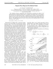
Figure 2 shows <strong>the</strong> result<strong>in</strong>g <strong>phase</strong> boundary for <strong>the</strong> <strong>Hubbard</strong><br />
<strong>model</strong> us<strong>in</strong>g <strong>the</strong> modified Stoner criterion. At halffill<strong>in</strong>g<br />
<strong>the</strong> transition is always commensurate with <strong>the</strong> lattice,<br />
i.e., q(/a)(1,1,1). As <strong>the</strong> system is doped away from<br />
half-fill<strong>in</strong>g <strong>the</strong> transition temperature decreases and a po<strong>in</strong>t is<br />
reached where <strong>the</strong> transition becomes <strong>in</strong>commensurate with<br />
<strong>the</strong> underly<strong>in</strong>g lattice. F<strong>in</strong>ite-size calculations show that <strong>the</strong><br />
order<strong>in</strong>g wave vector changes only along <strong>the</strong> Brillou<strong>in</strong> zone<br />
edge as <strong>the</strong> transition becomes <strong>in</strong>commensurate, i.e.,<br />
q(/a)(1,1,1) . The <strong>in</strong>set to Fig. 2 shows that rema<strong>in</strong>s<br />
small and eventually stops chang<strong>in</strong>g as <strong>the</strong> fill<strong>in</strong>g is
55 MAGNETIC PHASE DIAGRAM OF THE HUBBARD MODEL IN . . .<br />
945<br />
FIG. 2. <strong>Magnetic</strong> <strong>phase</strong> boundaries for <strong>the</strong> second-order local<br />
approximation to <strong>the</strong> <strong>Hubbard</strong> <strong>model</strong> <strong>in</strong> <strong>three</strong> <strong>dimensions</strong> for two<br />
different values <strong>of</strong> <strong>the</strong> <strong>in</strong>teraction strength U. The vertical axis<br />
shows <strong>the</strong> ratio <strong>of</strong> <strong>the</strong> temperature to <strong>the</strong> hopp<strong>in</strong>g constant. The<br />
horizontal axis shows <strong>the</strong> electron fill<strong>in</strong>g. The dashed solid l<strong>in</strong>es<br />
denote <strong>the</strong> <strong>in</strong>commensurate transition from a paramagnetic to a<br />
sp<strong>in</strong>-density-wave ground state <strong>in</strong> <strong>the</strong> <strong>the</strong>rmodynamic limit. The<br />
open solid circles denote <strong>the</strong> correspond<strong>in</strong>g transitions for a f<strong>in</strong>ite<br />
lattice <strong>of</strong> 80 unit cells for T0.05t and 500 unit cells for lower<br />
temperatures. The <strong>in</strong>set shows <strong>the</strong> correspond<strong>in</strong>g z component <strong>of</strong><br />
<strong>the</strong> magnetic order<strong>in</strong>g wave vector q vs fill<strong>in</strong>g. The <strong>phase</strong> <strong>diagram</strong><br />
is symmetric around n e 0.5.<br />
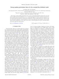
FIG. 3. <strong>Magnetic</strong> <strong>phase</strong> boundaries for <strong>the</strong> first-order approximation<br />
to <strong>the</strong> <strong>Hubbard</strong> <strong>model</strong> <strong>in</strong> <strong>three</strong> <strong>dimensions</strong> for two different<br />
values <strong>of</strong> <strong>the</strong> <strong>in</strong>teraction strength U. The vertical axis shows <strong>the</strong><br />
ratio <strong>of</strong> <strong>the</strong> temperature to <strong>the</strong> hopp<strong>in</strong>g constant. The horizontal axis<br />
shows <strong>the</strong> electron fill<strong>in</strong>g. The open solid circles denote <strong>the</strong> <strong>in</strong>-<br />
commensurate transition from a paramagnetic to a sp<strong>in</strong>-densitywave<br />
ground state for a f<strong>in</strong>ite lattice <strong>of</strong> 30 unit cells. The l<strong>in</strong>es are<br />
a guide to <strong>the</strong> eye. The <strong>in</strong>set shows <strong>the</strong> correspond<strong>in</strong>g z component<br />
<strong>of</strong> <strong>the</strong> magnetic order<strong>in</strong>g wave vector q vs fill<strong>in</strong>g. The <strong>phase</strong> <strong>diagram</strong><br />
is symmetric around n e 0.5.<br />
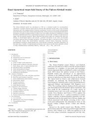
FIG. 4. Comparison between <strong>the</strong> results <strong>of</strong> quantum Monte<br />
Carlo simulations Ref. 10 circles, <strong>the</strong> first-order dashed l<strong>in</strong>e,<br />
and <strong>the</strong> second-order local approximation solid l<strong>in</strong>e. T c /t is <strong>the</strong><br />
ratio <strong>of</strong> <strong>the</strong> transition temperature at half-fill<strong>in</strong>g to <strong>the</strong> hopp<strong>in</strong>g <strong>in</strong>tegral.<br />
U is <strong>the</strong> <strong>in</strong>teraction strength. The second-order local approximation<br />
shows <strong>the</strong> same sign <strong>of</strong> <strong>the</strong> curvature as <strong>the</strong> QMC result,<br />
whereas <strong>the</strong> first-order curve shows <strong>the</strong> wrong sign <strong>of</strong> <strong>the</strong> curvature.<br />
Also, s<strong>in</strong>ce <strong>the</strong> second-order approximation has <strong>the</strong> correct limit<strong>in</strong>g<br />
behavior as U→0, this shows that <strong>the</strong> QMC data are overestimat<strong>in</strong>g<br />
T c for small values <strong>of</strong> U.<br />
changed. Note that <strong>the</strong> order<strong>in</strong>g wave vector <strong>in</strong>itially changes<br />
very rapidly at <strong>the</strong> <strong>in</strong>commensurate order onset, which is<br />
rem<strong>in</strong>iscent <strong>of</strong> <strong>the</strong> first-order jump seen <strong>in</strong> <strong>the</strong> Cr data. 1<br />
Figure 3 shows <strong>the</strong> result <strong>of</strong> a f<strong>in</strong>ite-size calculation for<br />
<strong>the</strong> orig<strong>in</strong>al Stoner criterion which results from a first-order<br />
Hartree approximation for <strong>the</strong> self-energy. We see that <strong>the</strong><br />
transition temperature is enhanced by almost a factor <strong>of</strong> 4 for<br />
each value <strong>of</strong> U compared to <strong>the</strong> second-order approximation<br />
results at half-fill<strong>in</strong>g. For a given value <strong>of</strong> U <strong>the</strong> change<br />
<strong>in</strong> slope at <strong>the</strong> onset <strong>of</strong> <strong>in</strong>commensuration is much smaller<br />
than <strong>the</strong> results <strong>of</strong> <strong>the</strong> second-order approximation. This<br />
change <strong>of</strong> slope <strong>in</strong> <strong>the</strong> second-order approximation is aga<strong>in</strong><br />
similar to what is seen <strong>in</strong> <strong>the</strong> Cr data. Also, as was already<br />
shown by Penn, 2 <strong>in</strong> <strong>the</strong> first-order approximation, for values<br />
<strong>of</strong> U large enough, <strong>the</strong> order<strong>in</strong>g wave vector changes first<br />
along <strong>the</strong> edge <strong>of</strong> <strong>the</strong> zone, but <strong>the</strong>n cont<strong>in</strong>ues to move toward<br />
<strong>the</strong> zone center as <strong>the</strong> system is doped far away from<br />
half-fill<strong>in</strong>g. This latter behavior has suggested that <strong>the</strong> system<br />
can become ferromagnetic for low electron fill<strong>in</strong>g which<br />
is ruled out once <strong>the</strong> quantum fluctuations are <strong>in</strong>cluded.<br />
Figure 4 shows a comparison <strong>of</strong> <strong>the</strong> transition temperature<br />
versus U at half-fill<strong>in</strong>g for <strong>the</strong> first- and second-order approximations<br />
as well as <strong>the</strong> result <strong>of</strong> a QMC simulation. 10<br />
We see that <strong>in</strong> <strong>the</strong> case <strong>of</strong> <strong>the</strong> second-order approximation,<br />
T c has negative curvature for U/t around 10 similar to <strong>the</strong><br />
QMC result although <strong>the</strong> former is not a valid approximation<br />
for large values <strong>of</strong> U), whereas <strong>in</strong> <strong>the</strong> first-order approximation<br />
T c cont<strong>in</strong>ues to <strong>in</strong>crease with U with a positive<br />
curvature. In fact, s<strong>in</strong>ce <strong>the</strong> second-order approximation is<br />
exact as U→0, it is clear that <strong>the</strong> QMC data are overestimat<strong>in</strong>g<br />
T c by a factor <strong>of</strong> 4 <strong>in</strong> <strong>the</strong> weak-coupl<strong>in</strong>g limit. Such<br />
criticism has already been raised by compar<strong>in</strong>g to o<strong>the</strong>r approximation<br />
methods. 11<br />
Electronic band structure calculations 1 show that <strong>the</strong><br />
d-electron concentration for pure Cr is 2.28 electrons/atom<br />
sp<strong>in</strong>. In order to map this onto our s<strong>in</strong>gle-band <strong>model</strong>, we<br />
assume that 1/5 <strong>of</strong> this contributes to our s<strong>in</strong>gle-band fill<strong>in</strong>g,<br />
imply<strong>in</strong>g n e 0.456 <strong>the</strong>re are five d bands <strong>in</strong> Cr. The Fermi<br />
energy <strong>of</strong> pure Cr is near <strong>the</strong> edge <strong>of</strong> a d band so that <strong>the</strong><br />
density <strong>of</strong> states has a large peak <strong>the</strong>re; thus we assume that<br />
dop<strong>in</strong>g with Mn adds one electron to <strong>the</strong> s<strong>in</strong>gle band and that<br />
dop<strong>in</strong>g with V removes one electron from it. This maps <strong>the</strong><br />
rest <strong>of</strong> <strong>the</strong> experimental data to <strong>the</strong> s<strong>in</strong>gle-band <strong>model</strong>. We<br />
<strong>the</strong>n fit <strong>the</strong> value <strong>of</strong> U <strong>in</strong> <strong>the</strong> modified Stoner criterion, to<br />
reproduce <strong>the</strong> experimental fill<strong>in</strong>g for <strong>the</strong> onset <strong>of</strong> <strong>in</strong>commensurate<br />
order. As shown <strong>in</strong> Fig. 5, <strong>the</strong> fit is remarkably<br />
good for U5.5t. Note that <strong>the</strong>re is only one adjustable<br />
parameter <strong>in</strong> this fit. The agreement is remarkable s<strong>in</strong>ce <strong>the</strong><br />
lattice structure for Cr is actually bcc and because we made<br />
such simple assumptions <strong>in</strong> <strong>the</strong> mapp<strong>in</strong>g to a s<strong>in</strong>gle-band<br />
<strong>model</strong>. Fur<strong>the</strong>rmore, <strong>the</strong> experimental shape cannot be properly<br />
accounted for with a first-order approximation for any<br />
reasonable value <strong>of</strong> U.<br />
V. CONCLUSIONS<br />
We found a criterion for <strong>the</strong> <strong>in</strong>stability <strong>of</strong> <strong>the</strong> paramagnetic<br />
ground state <strong>of</strong> <strong>the</strong> 3D <strong>Hubbard</strong> <strong>model</strong> towards <strong>the</strong>
946 A. N. TAHVILDAR-ZADEH, J. K. FREERICKS, AND M. JARRELL<br />
55<br />
FIG. 5. Comparison between <strong>the</strong> experimental data for chromium<br />
alloys Ref. 1 and <strong>the</strong> results <strong>of</strong> <strong>the</strong> second-order local approximation.<br />
The open solid circles denote <strong>the</strong> experimental data<br />
for <strong>the</strong> <strong>in</strong>commensurate transitions <strong>in</strong> Cr alloys. The dashed<br />
solid l<strong>in</strong>es denote <strong>the</strong> results <strong>of</strong> <strong>the</strong> second-order local approximation<br />
for <strong>the</strong> <strong>in</strong>commensurate transitions. The experimental data is<br />
best fit to <strong>the</strong> <strong>the</strong>oretical calculation when U5.5t. T I is <strong>the</strong><br />
transition temperature at <strong>the</strong> paramagnetic-commensurate<strong>in</strong>commensurate<br />
<strong>phase</strong> boundary. T I 360 K for experimental data<br />
and occurs when Cr is doped with 0.3 at. % <strong>of</strong> Mn.<br />
formation <strong>of</strong> an ordered SDW state. This criterion is a simple<br />
modification <strong>of</strong> <strong>the</strong> Stoner criterion and is derived by <strong>in</strong>clud<strong>in</strong>g<br />
<strong>the</strong> second-order graph <strong>in</strong> <strong>the</strong> expansion <strong>of</strong> <strong>the</strong> local selfenergy.<br />
Hence this criterion <strong>in</strong>cludes <strong>the</strong> lowest-order corrections<br />
<strong>of</strong> <strong>the</strong> old Stoner criterion due to quantum fluctuations.<br />
We showed that <strong>the</strong> magnetic <strong>phase</strong> boundary between<br />
<strong>the</strong> paramagnetic and SDW <strong>phase</strong>s <strong>of</strong> <strong>the</strong> <strong>model</strong> changes<br />
both quantitatively and qualitatively when we <strong>in</strong>clude <strong>the</strong><br />
effect <strong>of</strong> quantum fluctuations to <strong>the</strong> usual mean-field Hartree<br />
result. The quantum fluctuations suppress <strong>the</strong> transition<br />
temperatures and exclude <strong>the</strong> possibility <strong>of</strong> <strong>the</strong> formation <strong>of</strong><br />
ferromagnetism <strong>in</strong> <strong>the</strong> 3D <strong>Hubbard</strong> <strong>model</strong>.<br />
We showed that <strong>the</strong> result<strong>in</strong>g <strong>phase</strong> boundary from this<br />
modified Stoner criterion is consistent with <strong>the</strong> experimental<br />
data for <strong>the</strong> SDW <strong>in</strong> dilute chromium alloys whereas <strong>the</strong>re<br />
are features <strong>in</strong> <strong>the</strong> data that cannot be accounted for by <strong>the</strong><br />
usual Stoner criterion with reasonable values <strong>of</strong> <strong>the</strong> <strong>in</strong>teraction<br />
strength. We were <strong>in</strong>deed able to achieve remarkable<br />
agreement with <strong>the</strong> experimental data, although this <strong>model</strong> is<br />
too simple to be a realistic one for Cr. However, s<strong>in</strong>ce <strong>the</strong><br />
modified Stoner criterion is a simple and efficient approximation,<br />
we hope it can be applied to more realistic <strong>model</strong>s<br />
for Cr and o<strong>the</strong>r transition metals.<br />
ACKNOWLEDGMENTS<br />
We would like to acknowledge useful conversations with<br />
R. Fishman and P. van Dongen. This work was supported at<br />
<strong>the</strong> University <strong>of</strong> C<strong>in</strong>c<strong>in</strong>nati by <strong>the</strong> National Science Foundation<br />
Grants Nos. DMR-9406678 and DMR-9357199.<br />
J.K.F. acknowledges <strong>the</strong> Donors <strong>of</strong> The Petroleum Research<br />
Fund, adm<strong>in</strong>istered by <strong>the</strong> American Chemical Society, for<br />
support <strong>of</strong> this research ACS-PRF No. 29623-GB6.<br />
1 E. Fawcett, Rev. Mod. Phys. 60, 209 1988, and references<br />
<strong>the</strong>re<strong>in</strong>.<br />
2 D. R. Penn, Phys. Rev. 142, 350 1966.<br />
3 W. Metzner and D. Vollhardt, Phys. Rev. Lett. 62, 324 1989.<br />
4 P. G. J. van Dongen, Phys. Rev. Lett. 67, 757 1991.<br />
5 M. Jarrell, Phys. Rev. Lett. 69, 168 1992.<br />
6 J. K. Freericks and M. Jarrell, Phys. Rev. Lett. 74, 186 1995.<br />
7 J. K. Freericks and D. J. Scalap<strong>in</strong>o, Phys. Rev. B 49, 6368<br />
1994.<br />
8 J. <strong>Hubbard</strong>, Proc. R. Soc. London A 276, 238 1963.<br />
9 H. Schweitzer and G. Czycholl, Z. Phys. B 83, 931991.<br />
10 R. T. Scalettar, D. J. Scalap<strong>in</strong>o, R. L. Sugar, and D. Toussa<strong>in</strong>t,<br />
Phys. Rev. B 39, 4711 1989.<br />
11 Y. Kakehashi and H. Hasegawa, Phys. Rev. B 37, 7777 1988.