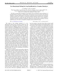
Exact dynamical mean-field theory of the Falicov-Kimball model

Exact dynamical mean-field theory of the Falicov-Kimball model 

J. K. Freericks* 

Department of Physics, Georgetown University, Washington, D.C. 20057, USA 

V. Zlatić † 

Institute of Physics, Bijenička cesta 46, P.O. Box 304, HR-10001, Zagreb, Croatia 

(Published 30 October 2003) 

REVIEWS OF MODERN PHYSICS, VOLUME 75, OCTOBER 2003 

The Falicov-Kimball model was introduced in 1969 as a statistical model for metal-insulator 

transitions; it includes itinerant and localized electrons that mutually interact with a local Coulomb 

interaction and is the simplest model of electron correlations. It can be solved exactly with dynamical 

mean-field theory in the limit of large spatial dimensions, which provides an interesting benchmark for 

the physics of locally correlated systems. In this review, the authors develop the formalism for solving 

the Falicov-Kimball model from a path-integral perspective and provide a number of expressions for 

single- and two-particle properties. Many important theoretical results are examined that show the 

absence of Fermi-liquid features and provide a detailed description of the static and dynamic 

correlation functions and of transport properties. The parameter space is rich and one finds a variety 

of many-body features like metal-insulator transitions, classical valence fluctuating transitions, 

metamagnetic transitions, charge-density-wave order-disorder transitions, and phase separation. At 

the same time, a number of experimental systems have been discovered that show anomalies related 

to Falicov-Kimball physics [including YbInCu 4 , EuNi 2 (Si 1x Ge x ) 2 ,NiI 2 , and Ta x N]. 

CONTENTS 

I. Introduction 1333 

A. Brief history 1333 

B. Hamiltonian and its symmetries 1335 

C. Outline of the review 1336 

II. Formalism 1337 

A. Limit of infinite spatial dimensions 1337 

B. Single-particle properties (itinerant electrons) 1338 

C. Static charge, spin, or superconducting order 1342 

D. Dynamical charge susceptibility 1345 

E. Static and dynamical transport 1348 

F. Single-particle properties (localized electrons) 1353 

G. Spontaneous hybridization 1356 

III. Analysis of Solutions 1356 

A. Charge-density-wave order and phase separation 1356 

B. Mott-like metal-insulator transitions 1360 

C. Falicov-Kimball-like metal-insulator transitions 1361 

D. Intermediate valence 1362 

E. Transport properties 1363 

F. Magnetic-field effects 1364 

G. Static Holstein model 1365 

IV. Comparison with Experiment 1366 

A. Valence-change materials 1366 

B. Electronic Raman scattering 1371 

C. Josephson junctions 1372 

D. Resistivity saturation 1373 

E. Pressure-induced metal-insulator transitions 1374 

V. New Directions 1374 

A. 1/d corrections 1374 

B. Hybridization and f-electron hopping 1377 

C. Nonequilibrium effects 1377 

VI. Conclusions 1378 

*Electronic address: freericks@physics.georgetown.edu; 

URL: http://www.physics.georgetown.edu/jkf 

† Electronic address: zlatic@ifs.hr 

Acknowledgments 1378 

List of Symbols 1379 

References 1379 

I. INTRODUCTION 

A. Brief history 

The Falicov-Kimball model (Falicov and Kimball, 

1969) was introduced in 1969 to describe metal-insulator 

transitions in a number of rare-earth and transitionmetal 

compounds [but see Hubbard’s earlier work (Hubbard, 

1963) where the spinless version of the Falicov- 

Kimball model was introduced as an approximate 

solution to the Hubbard model; one assumes that one 

species of spin does not hop and is frozen on the lattice]. 

The initial work by Falicov and collaborators focused 

primarily on analyzing the thermodynamics of the 

metal-insulator transition with a static mean-field-theory 

approach (Falicov and Kimball, 1969; Ramirez et al., 

1970). The resulting solutions displayed both continuous 

and discontinuous metal-insulator phase transitions, and 

they could fit the conductivity of a wide variety of 

transition-metal and rare-earth compounds with their 

results. Next, Ramirez and Falicov (1971) applied the 

model to describe the phase transition in cerium. 

Again, a number of thermodynamic quantities were approximated 

well by the model, but it did not display any 

effects associated with Kondo screening of the f electrons 

[and subsequently was discarded in favor of the 

Kondo volume collapse picture (Allen and Martin, 

1982)]. 

Interest in the model waned once Plischke (1972) 

showed that when the coherent-potential approximation 

(Soven, 1967; Velický et al., 1968) was applied to it, all 

first-order phase transitions disappeared and the solu- 

0034-6861/2003/75(4)/1333(50)/$35.00 1333 

©2003 The American Physical Society

1334 J. K. Freericks and V. Zlatić: Exact dynamical mean-field theory of the Falicov-Kimball model 

tions only displayed smooth crossovers from a metal to 

an insulator [this claim was strongly refuted by Falicov’s 

group (Gonçalves da Silva and Falicov, 1972) but interest 

in the model was limited for almost 15 years]. 

The field was revitalized by mathematical physicists in 

the mid 1980s, who realized that the spinless version of 

this model is the simplest correlated electronic system 

that displays long-range order at low temperatures and 

for dimensions greater than one. Indeed, two groups 

produced independent proofs of the long-range order 

(Brandt and Schmidt, 1986, 1987; Kennedy and Lieb, 

1986; Lieb, 1986). In their work, Kennedy and Lieb rediscovered 

Hubbard’s original approximation that yields 

the spinless Falicov-Kimball (FK) model, and also provided 

a new interpretation of the model for the physics 

of crystallization. A number of other exact results followed 

including (i) a proof of no quantum-mechanical 

mixed valence (or spontaneous hybridization) at finite T 

(Subrahmanyam and Barma, 1988) based on the presence 

of a local gauge symmetry and Elitzur’s theorem 

(Elitzur, 1975); (ii) proofs of phase separation and of 

periodic ordering in one dimension (with large interaction 

strength; Lemberger, 1992); (iii) proofs about 

ground-state properties in two dimensions (also at large 

interaction strength; Kennedy, 1994, 1998; Haller, 2000; 

Haller and Kennedy, 2001); (iv) a proof of phase separation 

in one dimension and small interaction strength 

(Freericks et al., 1996); and (v) a proof of phase separation 

for large interaction strength and all dimensions 

(Freericks et al., 2002a, 2002b). Most of these rigorous 

results have already been summarized in reviews (Gruber 

and Macris, 1996; Gruber, 1999). In addition, a series 

of numerical calculations were performed in one and 

two dimensions (Freericks and Falicov, 1990; de Vries 

et al., 1993, 1994; Michielsen, 1993; Gruber et al., 1994; 

Watson and Lemański, 1995; Lemański, Freericks, and 

Banach, 2002). While not providing complete results for 

the model, the numerics do illustrate a number of important 

trends in the physics of the FK model. 

At about the same time, there was a parallel development 

of the dynamical mean-field theory (DMFT), 

which is what we concentrate on in this review. The 

DMFT was invented by Metzer and Vollhardt (1989). 

Almost immediately after the idea that in large spatial 

dimensions the self-energy becomes local, Brandt and 

collaborators showed how to solve the static problem 

exactly (requiring no quantum Monte Carlo), thereby 

providing the exact solution of the Falicov-Kimball 

model (Brandt and Mielsch, 1989, 1990, 1991; Brandt 

et al., 1990; Brandt and Fledderjohann, 1992; Brandt and 

Urbanek, 1992). This work is the extension of Onsager’s 

famous solution for the transition temperature of the 

two-dimensional Ising model to the fermionic case (and 

large dimensions). These series of papers revolutionized 

Falicov-Kimball-model physics and provided the only 

exact quantitative results for electronic phase transitions 

in the thermodynamic limit for all values of the interaction 

strength. They showed how to solve the infinitedimensional 

DMFT model, illustrated how to determine 

the order-disorder transition temperature for a checkerboard 

(and incommensurate) charge-density-wave 

phase, showed how to find the free energy (including a 

first study of phase separation), examined properties of 

the spin-one-half model, and calculated the f-particle 

spectral function. 

Further work concentrated on static properties such 

as charge-density-wave order (van Dongen and Vollhardt, 

1990; van Dongen, 1991a, 1992; Freericks, 1993a, 

1993b; Gruber et al., 2001; Chen, Jones, and Freericks, 

2003) and phase separation (Freericks et al., 1999; Letfulov, 

1999; Freericks and Lemański, 2000). The original 

Falicov-Kimball problem of the metal-insulator transition 

(Chung and Freericks, 1998) was solved, as was the 

problem of classical intermediate valence (Chung and 

Freericks, 2000), both using the spin-one-half generalization 

(Brandt et al., 1990; Freericks and Zlatić, 1998). 

The ‘‘Mott-like’’ metal-insulator transition (van Dongen 

and Leinung, 1997; Kalinowski and Gebhard, 2002) and 

the non-Fermi-liquid behavior (Si et al., 1992) were also 

investigated. Dynamical properties and transport have 

been determined ranging from the charge susceptibility 

(Freericks and Miller, 2000; Shvaika, 2000, 2001), to the 

optical conductivity (Moeller et al., 1992), to the Raman 

response (Freericks and Devereaux, 2001a, 2001b; 

Freericks, Devereaux, and Bulla, 2001; Devereaux et al., 

2003a, 2003b), to an evaluation of the f spectral function 

(Brandt and Urbanek, 1992; Si et al., 1992; Zlatić et al., 

2001). Finally, the static susceptibility for spontaneous 

polarization was also determined (Subrahmanyam and 

Barma, 1988; Si et al., 1992; Portengen et al., 1996a, 

1996b; Zlatić et al., 2001). 

These solutions have allowed the FK model to be applied 

to a number of different experimental systems 

ranging from valence-change-transition materials (Zlatić 

and Freericks, 2001a, 2001b, 2003a, 2003b) like YbInCu 4 

and EuNi 2 (Si 1x Ge x ) 2 , to materials that can be doped 

through a metal-insulator transition like Ta x N [used as a 

barrier in Josephson junctions (Freericks, Nikolić, and 

Miller, 2001, 2002, 2003a, 2003b, 2003c; Miller and Freericks, 

2001)], to Raman scattering in materials on the 

insulating side of the metal-insulator transition (Freericks 

and Devereaux, 2001b) like FeSi or SmB 6 . The 

model, and some straightforward modifications appropriate 

for double exchange, has been used to describe 

the colossal magnetoresistance materials (Allub and 

Alascio, 1996, 1997; Letfulov and Freericks, 2001; 

Ramakrishnan et al., 2003). 

Generalizations of the FK model to the static Holstein 

model were first carried out by Millis et al. (1995, 1996) 

and also applied to the colossal magnetoresistance materials. 

Later more fundamental properties were worked 

out, relating to the transition temperature for the harmonic 

(Ciuchi and de Pasquale, 1999; Blawid and Millis, 

2000) and anharmonic cases (Freericks et al., 2000), and 

relating to the gap ratio for the harmonic (Blawid and 

Millis, 2001) and anharmonic cases (Freericks and Zlatić, 

2001a). Modifications to examine diluted magnetic 

semiconductors have also appeared (Chattopadhyay 

et al., 2001; Hwang et al., 2002). A new approach to 

DMFT, which allows the correlated hopping Falicov- 

Kimball model to be solved has also been presented recently 

(Schiller, 1999; Shvaika, 2003). 

Rev. Mod. Phys., Vol. 75, No. 4, October 2003

J. K. Freericks and V. Zlatić: Exact dynamical mean-field theory of the Falicov-Kimball model 

1335 

B. Hamiltonian and its symmetries 

The Falicov-Kimball model is the simplest model of 

correlated electrons. The original version (Falicov and 

Kimball, 1969) involved spin-one-half electrons. Here, 

we shall generalize to the case of an arbitrary degeneracy 

of the itinerant and localized electrons. The general 

Hamiltonian is then 

Ht 

ij 

U 

i 

 

i 

2s1 

2S1 

1 

c † i c j 

i 1 

E f f † i f i 

2s1 

1 

 

2S1 

 

1 

2S1 

1 

ff 

U 

f i 

c † i c i f † i f i 

† 

† f i f i f i 

2s1 

g B H 

i 1 

m c † i c i 

2S1 

g f B H 

i 1 

m f † i f i . (1) 

† 

The symbols c i and c i denote the itinerant-electron 

creation and annihilation operators, respectively, at site i 

in state (the index takes 2s1 values). Similarly, the 

† 

symbols f i and f i denote the localized-electron creation 

and annihilation operators at site i in state (the 

index takes 2S1 values). Customarily, we identify 

the index and with the z component of spin, but the 

index could denote other quantum numbers in more 

general cases. The first term is the kinetic energy (hopping) 

of the conduction electrons (with t denoting the 

nearest-neighbor hopping integral); the summation is 

over nearest-neighbor sites i and j (we count each pair 

twice to guarantee hermiticity). The second term is the 

localized-electron site energy, which we allow to depend 

on the index to include crystal-field effects (without 

spin-orbit coupling for simplicity); in most applications 

the site energy is taken to be independent. The third 

term is the Falicov-Kimball interaction term (of strength 

U), which represents the local Coulomb interaction 

when itinerant and localized electrons occupy the same 

lattice site. We could make U depend on or , but this 

complicates the formulas and is not normally needed. 

The fourth term is the ff Coulomb interaction energy of 

ff 

strength U 

, which can be chosen to depend on if 

desired; the term with is unnecessary and can be 

absorbed into E f . Finally, the fifth and sixth terms represent 

the magnetic energy due to the interaction with 

an external magnetic field H, with B the Bohr magneton, 

g (g f ) the respective Landé g factors, and m (m ) 

the z component of spin for the respective states. 

Chemical potentials and f are employed to adjust the 

itinerant- and localized-electron concentrations by subtracting 

N and f N f , respectively, from H (in cases 

where the localized particle is fixed independently of the 

itinerant-electron concentration, the localized-particle 

chemical potential f can be absorbed into the site energy 

E f ; in cases where the localized particles are electrons, 

they share a common chemical potential with the 

conduction electrons f ). 

The spinless case corresponds to the case in which s 

S0 and there is no ff interaction term because of the 

Pauli exclusion principle. The original Falicov-Kimball 

model corresponds to the case in which sS1/2, with 

spin-one-half electrons for both itinerant and localized 

cases (and the limit U ff →). 

The Hamiltonian in Eq. (1) possesses a number of 

different symmetries. The partial particle-hole symmetry 

holds on a bipartite lattice in no magnetic field (H 

0), where the lattice sites can be organized into two 

sublattices A and B, and the hopping integral only connects 

different sublattices. In this case, one performs a 

partial particle-hole symmetry transformation on either 

the itinerant or localized electrons (Kennedy and Lieb, 

1986). The transformation includes a phase factor of 

(1) for electrons on the B sublattice. When the partial 

particle-hole transformation is applied to the itinerant 

electrons, 

c i →c h† i 1 p(i) , (2) 

with p(i)0 for iA and p(i)1 for iB and h denoting 

the hole operators, then the Hamiltonian maps 

onto itself (when expressed in terms of the hole operators 

for the itinerant electrons), up to a numerical shift, 

with U→U, E f →E f U, and →. When applied 

to the localized electrons, 

f i →f h† i 1 p(i) , (3) 

the Hamiltonian maps onto itself (when expressed in 

terms of the hole operators for the localized electrons), 

up to a numerical shift with U→U, →U, E f 

ff 

ff 

→E f U 

U 

, and f → f . 

These particle-hole symmetries are particularly useful 

ff 

when E f 0, U 

does not depend on , and we 

work in the canonical formalism with fixed values of e 

and f , the total itinerant- and localized-electron densities. 

Then, one can show that the ground-state energies 

of H are simply related, 

E g.s. e , f ,UE g.s. 2s1 e , f ,U 

E g.s. e ,2S1 f ,U 

E g.s. 2s1 e ,2S1 f ,U (4) 

(up to constant shifts or shifts proportional to e or f ), 

and one can restrict the phase space to e s 1 2 and f 

S 1 2 . 

When one or more of the Coulomb interactions are 

infinite, there are additional symmetries to the Hamiltonian 

(Freericks et al., 1999, 2002b). When all U 

ff 

, then we are restricted to the subspace f 1. This 

system is formally identical to the case of spinless localized 

electrons, and we shall develop a full solution of 

this limit using DMFT below. The extra symmetry is precisely 

that of Eq. (4), but now with S0 (regardless of 

ff 

the number of states). Similarly, when both U 

and U, then Eq. (4) holds for sS0 as well 



(regardless of the number of and states). These 

infinite-U symmetries are also related to particle-hole 

symmetry, but now restricted to the lowest Hubbard 

band in the system, since all upper Hubbard bands are 

pushed out to infinite energy. 

The Falicov-Kimball model also possesses a local symmetry, 

related to the localized particles. One can easily 

show that H,f † i f i 0, implying that the local occupancy 

of the f electrons is conserved. Indeed, this leads 

to a local U(1) symmetry, as the phase of the localized 

electrons can be rotated at will, without any effect on 

the Hamiltonian. Because of this local gauge symmetry, 

Elitzur’s theorem requires that there be no quantummechanical 

mixing of the f-particle number at finite temperature 

(Elitzur, 1975; Subrahmanyam and Barma, 

1988), hence the system can never develop a spontaneous 

hybridization (except possibly at T0). 

There are a number of different ways to provide a 

physical interpretation of the Falicov-Kimball model. In 

the original idea (Falicov and Kimball, 1969), we think 

of having itinerant and localized electrons that can 

change their statistical occupancy as a function of temperature 

(maintaining a constant total number of electrons). 

This is the interpretation that leads to a metalinsulator 

transition due to the change in the occupancy 

of the different electronic levels, rather than via a 

change in the character of the electronic states themselves 

(the Mott-Hubbard approach). Another interpretation 

(Kennedy and Leib, 1986) is to consider the localized 

particles as ions, which have an attractive 

interaction with the electrons. Then one can examine 

how the Pauli principle forces the system to minimize its 

energy by crystallizing into a periodic arrangement of 

ions and electrons (as seen in nearly all condensedmatter 

systems at low temperature). Finally, we can map 

onto a binary alloy problem (Freericks and Falicov, 

1990), where the presence of an ‘‘ion’’ denotes the A 

species, and the absence of an ‘‘ion’’ denotes a B species, 

with U becoming the difference in site energies for an 

electron on an A or a B site. In these latter two interpretations, 

the localized particle number is always a constant, 

and a canonical formalism is most appropriate. In 

the first interpretation, a grand canonical ensemble is 

the best approach, with a common chemical potential 

( f ) for the itinerant and localized electrons. 

In addition to the traditional Falicov-Kimball model, 

in which conduction electrons interact with a discrete set 

of classical variables (the localized electron-number operators), 

there is another class of static models that can 

be solved using the same kind of techniques—the static 

anharmonic Holstein model (Holstein, 1959; Millis et al., 

1995). This is a model of classical phonons interacting 

with conduction electrons and can be viewed as replacing 

the discrete spin variable of the FK model by a continuous 

classical field. The phonon is an Einstein mode, 

with infinite mass (and hence zero frequency), but nonzero 

spring constant. One can add any form of local anharmonic 

potential for the phonons into the system as 

well. The Hamiltonian becomes (in the spin-one-half 

case for the conduction electrons, with one phonon 

mode per site) 

H Hol t 

ij 

c † i c j g ep x i c † i c i e 

i 

1 2 

i 

x i 2 an 

i 

x i 3 an 

i 

x i 4 , (5) 

where, for concreteness, we assumed a quartic phonon 

potential. The phonon coordinate at site i is x i , g ep is 

the electron-phonon interaction strength (the so-called 

deformation potential), and the coefficients an and an 

measure the strength of the (anharmonic) cubic and 

quartic contributions to the local phonon potential. Note 

that the phonon couples to the fluctuations in the local 

electronic charge (rather than the total charge). This 

makes no difference for a harmonic system, where the 

shift in the phonon coordinate can always be absorbed, 

but it does make a difference for the anharmonic case, 

where such shifts cannot be transformed away. The 

particle-hole symmetry of this model is similar to that of 

the discrete Falicov-Kimball model, described above, 

except the particle-hole transformation on the phonon 

coordinate requires us to send x i →x i . Hence the presence 

of a cubic contribution to the phonon potential 

an 0 breaks the particle-hole symmetry of the system 

(Hirsch, 1993); in this case the phase diagram is not symmetric 

about half filling for the electrons. We shall discuss 

some results of the static Holstein model, but we 

shall not discuss any further extensions (such as including 

double exchange for colossal magnetoresistance materials 

or including interactions with classical spins to 

describe diluted magnetic semiconductors). 

C. Outline of the review 

The Falicov-Kimball model and the static Holstein 

model become exactly solvable in the limit of infinite 

spatial dimensions (or equivalently when the coordination 

number of the lattice becomes large). This occurs 

because both the self-energy and the (relevant) irreducible 

two-particle vertices are local. The procedure involves 

a mapping of the infinite-dimensional lattice 

problem onto a single-site impurity problem in the presence 

of a time-dependent (dynamical) mean field. The 

path integral for the partition function can be evaluated 

exactly via the so-called ‘‘static approximation’’ in an 

arbitrary time-dependent field. Hence the problem is reduced 

to one of ‘‘quadratures’’ to determine the correct 

self-consistent dynamical mean field for the quantum 

system. One can next employ the Baym-Kadanoff conserving 

approach to exactly determine the self-energies 

and the irreducible charge vertices (both static and dynamic). 

Armed with these quantities, one can calculate 

essentially all many-body correlation functions imaginable, 

ranging from static charge-density order to a dynamical 

Raman response. Finally, one can also calculate 

the properties of the f-electron spectral function, and 

with that, one can calculate the susceptibility for spon- 



1337 

taneous hybridization formation. The value of the 

Falicov-Kimball model lies in the fact that all of these 

many-body properties can be determined exactly and 

thereby form a useful benchmark for the properties of 

correlated electronic systems. 

In Sec. II, we review the formalism that develops the 

exact solution for all of these different properties employing 

DMFT. Our attempt is to provide all details of 

the most important derivations, and summarizing formulas 

for some of the more complicated results, which are 

treated fully in the literature. We believe that this review 

provides a useful starting point for interested researchers 

to understand that literature. Section III presents a 

summary of the results for a number of different properties 

of the model, concentrating mainly on the spinless 

and spin-one-half cases. In Sec. IV, we provide a number 

of examples in which the Falicov-Kimball model can be 

applied to model real materials, concentrating mainly on 

valence-change systems like YbInCu 4 . We discuss a 

number of interesting new directions in Sec. V, followed 

by our conclusions in Sec. VI. 

II. FORMALISM 

A. Limit of infinite spatial dimensions 

In 1989, Metzner and Vollhardt demonstrated that the 

many-body problem is simplified in the limit of large 

dimensions (Metzner and Vollhardt, 1989); equivalently, 

this observation could be noted to be a simplification 

when the coordination number Z on a lattice becomes 

large. Such ideas find their origin in the justification of 

the inverse coordination number 1/Z as the small parameter 

governing the convergence of the coherentpotential 

approximation (Schwartz and Siggia, 1972). 

Metzner and Vollhardt (1989) introduced an important 

scaling of the hopping matrix element, 

tt*/2dt*/2Z, (6) 

where d is the spatial dimension. In the limit where d 

→, the hopping to nearest neighbors vanishes, but the 

coordination number becomes infinite—this is the only 

scaling that produces a nontrivial electronic density of 

states in the large-dimensional limit. Since there is a 

noninteracting ‘‘band,’’ one can observe the effects of 

the competition of kinetic-energy delocalization with 

potential-energy localization, which forms the crux of 

the many-body problem. Hence this limit provides an 

example of exact solution of the many-body problem, 

and these solutions can be analyzed for correlatedelectron 

behavior. 

Indeed, the central-limit theorem shows that the noninteracting 

density of states on a hybercubic lattice 

hyp () satisfies (Metzner and Vollhardt, 1989) 

1 

hyp exp 2 /t* 2 , (7) 

t* uc 

which follows from the fact that the band structure is a 

sum of cosines, which are distributed between 1 and 1 

for a ‘‘general’’ wave vector in the Brillouin zone (here 

uc is the volume of the unit cell, which we normally 

take to be equal to 1). Adding together d cosines will 

produce a sum that typically grows like d, which is why 

the hopping is chosen to scale like 1/d. The centrallimit 

theorem then states that the distribution of these 

energies is in a Gaussian. [An alternate derivation relying 

on tight-binding Green’s functions and the properties 

of Bessel functions can be found in Müller-Hartmann 

(1989a).] Another common lattice that is examined is 

the infinite-coordination Bethe lattice, which can be 

thought of as the interior of a large Cayley tree. The 

noninteracting density of states is (Economou, 1983) 

1 

Bethe 

2t* 2 4t* 2 2 , (8) 

uc 

where we used the number of neighbors Z4d and the 

scaling in Eq. (6). 

The foundation for DMFT comes from two facts: first 

the self-energy is a local quantity, possessing temporal 

but not spatial fluctuations, and second it is a functional 

of the local interacting Green’s function. These observations 

hold for any ‘‘impurity’’ model as well, where the 

self-energy can be extracted by a functional derivative of 

the Luttinger-Ward skeleton expansion for the selfenergy 

generating functional (Luttinger and Ward, 

1960). Hence a solution of the impurity problem provides 

the functional relationship between the Green’s 

function and the self-energy. A second relationship is 

found from Dyson’s equation, which expresses the local 

Green’s function as a summation of the momentumdependent 

Green’s functions over all momenta in the 

Brillouin zone. Since the self-energy has no momentum 

dependence, this relation is a simple integral relation 

(called the Hilbert transformation) of the noninteracting 

density of states. Combining these two ideas in a selfconsistent 

fashion provides the basic strategy of DMFT. 

For the Falicov-Kimball model, we need to establish 

these two facts. The locality of the self-energy is established 

most directly from an examination of the perturbation 

series, where one can show nonlocal self-energies 

are smaller by powers of 1/d. The skeleton expansion 

for the self-energy (determined by the functional derivative 

of the Luttinger-Ward self-energy generating functional 

with respect to G), appears in Fig. 1 through 

fourth order in U. This expansion is identical to the expansion 

for the Hubbard model, except we explicitly 

note the localized and itinerant Green’s functions 

graphically. Since the localized-electron propagator is local, 

i.e., has no off-diagonal spatial components, many of 

the diagrams in Fig. 1 are also purely local. The only 

nonlocal diagrams through fourth order are the first diagrams 

in the second and third rows. If we suppose i and 

j correspond to nearest neighbors, then we immediately 

conclude that the diagram has three factors of G ij 

1/d 3 (each 1/d factor comes from t ij ). Summing 

over all of the 2d nearest neighbors still produces a result 

that scales like 1/d in the large-dimensional limit, 

which vanishes. A similar argument can be extended to 



c i e (HN) c i 0e (HN) , (10) 

and the trace is over all of the itinerant and localized 

electronic states. It is convenient to introduce a pathintegral 

formulation using Grassman variables ¯i () 

and i () for the itinerant electrons at site i with spin 

. Using the Grassman form for the coherent states then 

produces the path integral 

G ij 1 Z L 

Tr f e (H f f N f ) 

D¯D i ¯j 0e SL (11) 

FIG. 1. Skeleton expansion for the itinerant-electron selfenergy 

ij through fourth order. The wide solid lines denote 

itinerant-electron Green’s functions and the thin solid lines denote 

localized-electron Green’s functions; the dotted lines denote 

the Falicov-Kimball interaction U. The series is identical 

to that of the Hubbard model, except we must restrict the 

localized-electron propagator to be diagonal in real space 

(which reduces the number of off-diagonal diagrams significantly). 

The first diagrams in the second and third rows are the 

only diagrams that contribute when ij for the Falicov- 

Kimball model. 

all nonlocal diagrams (Brandt and Mielsch, 1989; 

Metzner, 1991). Hence the self-energy is local in the 

infinite-dimensional limit. The functional dependence 

on the local Green’s function then follows from the skeleton 

expansion, restricted to the local self-energy (i 

j). 

B. Single-particle properties (itinerant electrons) 

We start our analysis by deriving the set of equations 

satisfied by the single-particle lattice Green’s function 

for the itinerant electrons defined by the time-ordered 

product 

G ij 1 Tr 

Z cf e (HN f N f ) T c i c † j 0, 

L 

(9) 

where 1/T is the inverse temperature, 0 is the 

imaginary time, Z L is the lattice partition function, N is 

the total itinerant-electron number, N f is the total 

localized-electron number, and T denotes imaginary 

time ordering (earlier times to the right). The time dependence 

of the electrons is 

for the Green’s function, where H f denotes the 

f-electron-only piece of the Hamiltonian, corresponding 

to the second, fourth, and sixth terms in Eq. (1). The 

lattice action associated with the Hamiltonian in Eq. (1) 

is 

 

d¯i 

0 

S L 

ij 

ij 

2s1 

1 

 

 

t ij* 

2d ijUN fi g B Hm 

j , (12) 

with N fi the total number of f electrons at site i. Since 

the Grassman variables are antiperiodic on the interval 

0, we can expand them in Fourier modes, indexed 

by the fermionic Matsubara frequencies i n 

iT(2n1): 

 

i T e i n i i n (13) 

n 

and 

 

¯i T e i n ¯i i n . (14) 

n 

In terms of this new set of Grassman variables, the lattice 

action becomes S L 

T n S L n , with 

S n L 

ij 

2s1 

1 

 

i n g B Hm UN fi ij 

t ij* 

i n j i n (15) 

2d¯i 

and the Fourier component of the local Green’s function 

becomes 

G ii i n 

0 

 

de 

i n G ii 

T Z L 


D¯D i i n ¯i i n e T n S L 

n . 

(16) 



1339 

Now we are ready to begin the derivation of the 

DMFT equations for the Green’s functions. We start 

with the many-body-variant of the cavity method 

(Georges et al., 1996; Gruber et al., 2001), where we 

separate the path integral into pieces that involve site i 

only and all other terms. The action is then broken into 

three pieces: (i) the local piece at site i, S n (i,i); (ii) the 

piece that couples to site i, S n (i,j); and the piece that 

does not involve site i at all, S n (cavity), called the cavity 

piece. Hence 

S L n S n i,iS n i,jS n cavity (17) 

with 

2s1 

S n i,i 

1 

i n g B Hm UN fi 

¯i i n i i n , (18) 

and 

S n i,j 

j,t ij 

*0 

2s1 

1 

t ij 

* 

2d 

¯i i n j i n ¯j i n i i n , 

(19) 

S n cavityS n L S n i,iS n i,j. (20) 

Let Z cavity and cavity denote the partition function 

and path-integral average associated with the cavity action 

S cavity T n S n (cavity) (the path-integral average 

for the cavity is divided by the cavity partition function). 

Then the Green’s function can be written as 

G ii i n T Z cavity 

Z L 

exp T 

n 

Tr f e (H f f N f 

) D¯iD i i i n ¯i i n e T 

S 

n n (i,i) 

 

 

j,t ij 

*0 

2s1 

 

1 

t ij 

* 

2d ¯i i n j i n ¯j i n i i n cavity 

. (21) 

A simple power-counting argument shows that only the 

second moment of the exponential factor in the cavity 

average contributes as d→ (Georges et al., 1996), 

which then becomes 

G ii i n T Z cavity 

Z L 


D¯iD i i i n ¯i i n 

exp T 

 

 

n 

g B Hm UN fi 

2s1 

i n 

1 

i i n ¯i i n i i n , (22) 

with i (i n ) the function that results from the secondmoment 

average that is called the dynamical mean field. 

On a Bethe lattice, one finds i (i n )t* 2 G ii (i n ), 

while on a general lattice, one finds i (i n ) 

jk t ij t ik G jk (i n )G ji (i n )G ik (i n )/G ii (i n ) 

(Georges et al., 1996). But the exact form is not important 

for deriving the DMFT equations. Instead we simply 

need to note that after integrating over the cavity, we 

find an impurity path integral for the Green’s function 

(after defining the impurity partition function via Z imp 

Z L /Z cavity ), 

G ii i n ln Z imp 

i i n , 

Z imp Tr f e (H f f N f 

) D¯iD i 

2s1 

exp T 

n 

i n g B Hm 

1 

UN fi i i n ¯i i n i i n . (23) 

The impurity partition function is easy to calculate because 

the effective action is quadratic in the Grassman 

variables. Defining Z 0 () by 

 

Z 0 2e /2 n 

 

i n n 

i n 

, (24) 

where we used the notation n i (i n ) and adjusted 

the prefactor to give the noninteracting result, allows us 

to write the partition function as 

Z imp Tr f expH fi f N fi 

2s1 

 

1 

Z 0 g B Hm UN fi . (25) 

Here Z 0 (g B Hm ) is the generating functional for 

the U0 impurity problem and satisfies the relation 

Z 0 DetG 1 0 , with G 1 

0 defined below in frequency 

space in Eq. (29) and a proper regularization introduced 



to reproduce the 0 partition function. It is cumbersome 

to write out the trace over the fermionic states in 

Eq. (25) for the general case. The spin-one-half case appears 

in Brandt et al. (1990). Here we consider only the 

ff 

strong-interaction limit, where U →, so that there 

is no double occupancy of the f electrons. In this case we 

find 

Z imp 

1 

 

1 

Z 0 g B Hm U. (26) 

Evaluating the derivative yields 

with 

G n 

i n g B Hm n 

w 0 

1 

 

and w 1 1w 0 . The weight w 1 

f-electron concentration f . If we relaxed the restriction 

ff 

U →, then we would have additional terms corresponding 

to w i , with 1i2S1. Defining the effective 

medium (or bare Green’s function) via 

G 0 i n 1 i n g B Hm n (29) 

allows us to reexpress Eq. (27) as 

G n w 0 

G 0 

which is a form that often appears in the literature. Dyson’s 

equation for the impurity self-energy is 

n i n G 0 i n 1 G i n 1 . (31) 

This impurity self-energy is equated with the local selfenergy 

of the lattice (since they satisfy the same skeleton 

expansion with respect to the local Green’s function). 

We can calculate the local Green’s function directly from 

this self-energy by performing a spatial Fourier transform 

of the momentum-dependent Green’s function on 

the lattice: 

G n 

k 

1 

 

k i n g B Hm n k 

d 

1 

i n g B Hm n , (32) where k is the noninteracting band structure. This rela- 

2s1 

Z 0 g B Hm 

n 1 U 1 

2 G n 

U 1 

U 

G n 

24w 1 

G n, 

2S1 

(33) 

 

1 

e (E f f g f B Hm ) 

2s1 

w 0 

w 1 

 

i n g B Hm n U , (27) 

2s1 

Z 0 g B Hm /Z imp , (28) 

equals the average 

1 i n w 1 

G 0 i n U , (30) 

G n k 

tion is called the Hilbert transformation of the noninteracting 

density of states. Equating the Green’s function in 

Eq. (32) to that in Eq. (30) is the self-consistency relation 

of DMFT. Substituting Eq. (31) into Eq. (30) to 

eliminate the bare Green’s function produces a quadratic 

equation for the self-energy, solved by Brandt and 

Mielsch (1989, 1990), 

which is the exact summation of the skeleton expansion 

for the self-energy in terms of the interacting Green’s 

function (the sign in front of the square root is chosen to 

preserve the analyticity of the self-energy). Note that, 

because w 1 is a complicated functional of G n and n , 

Eq. (33) actually corresponds to a highly nonlinear functional 

relation between the Green’s function and the 

self-energy. 

There are two independent strategies that one can 

employ to calculate the FK-model Green’s functions. 

The original method of Brandt and Mielsch is to substitute 

Eq. (33) into Eq. (32), which produces a transcendental 

equation for G n in the complex plane (for fixed 

w 1 ; Brandt and Mielsch, 1989, 1990). This equation can 

be solved by a one-dimensional complex root-finding 

technique, typically Newton’s method or Mueller’s 

method, as long as one pays attention to maintaining the 

analyticity of the self-energy by choosing the proper sign 

for the square root. For large U, the sign changes at a 

critical value of the Matsubara frequency (Freericks, 

1993a). The other technique is the iterative technique 

first introduced by Jarrell (1992), which is the most commonly 

used method. One starts the algorithm either with 

n 0 or with it chosen appropriately from an earlier 

calculation. Evaluating Eq. (32) for G n then allows one 

to calculate G 0 from Eq. (31). If we work at fixed chemical 

potential and fixed E f , then we must determine w 0 

and w 1 from Eq. (28); this step is not necessary if w 0 and 

w 1 are fixed in a canonical ensemble. Equation (30) is 

employed to find the new Green’s function, and Eq. (31) 

is used to extract the new self-energy. The algorithm 

then iterates to convergence by starting with this new 

self-energy. Typically, the algorithm converges to eight 

decimal points in less than 100 iterations, but for some 

regions of parameter space the equations can either converge 

very slowly or not converge at all. Convergence 

can be accelerated by averaging the last iteration with 

the new result for determining the new self-energy, but 

there are regions of parameter space where the iterative 

technique does not appear to converge. 

Once w 0 , w 1 , and are known from the imaginaryaxis 

calculation, one can employ the analytic continuation 

of Eqs. (30)–(32) (with i n →i0 ) to calculate 

G () on the real axis. In general, the convergence is 

slower on the real axis than on the imaginary axis, with 

the spectral weight slowest to converge near correlationinduced 

‘‘band edges.’’ A stringent consistency test of 



1341 

this technique is a comparison of the Green’s function 

calculated directly on the imaginary axis to that found 

from the spectral formula 

G z d 

A 

zi0 , (34) 

with 

and 

A dA ,, (35) 

A , 1 Im 1 

g B Hm i0 (36) 

[the infinitesimal 0 is needed only when Im ()0]. 

Note that this definition of the interacting density of 

states has the chemical potential located at 0. 

In zero magnetic field, one need perform these calculations 

only for one state, since all G n ’s are equal, but 

in a magnetic field one must perform 2s1 parallel calculations 

to determine the G n ’s. 

Our derivation of the single-particle Green’s functions 

has followed a path-integral approach throughout. One 

could have used an equation-of-motion approach instead. 

This technique has been reviewed by Zlatić et al. 

(2001). 

The formalism for the static Holstein model is similar 

(Millis et al., 1996). Taking to be a continuous variable 

(x) and H0, we find 

and 

Z imp 

 

G n 

 

2s1 

 

dx 

1 

Z 0 g ep x 

exp 1 2 x2 an x 3 an x 4, (37) 

 

dx 

2s1 

wx 

1 

wx 

i n g ep x n 

, (38) 

Z 0 g ep x 

exp 1 2 x2 an x 3 an x 4 Z imp . 

(39) 

Equations (37)–(39) and Eqs. (31) and (32) are all that 

are needed to determine the Green’s functions by using 

the iterative algorithm. 

The final single-particle quantity of interest is the 

Helmholtz free energy per lattice site F Helm. . We restrict 

our discussion to the case of zero magnetic field 

H0 and to E f E f (no dependence to E f ). There 

are two equivalent ways to calculate the free energy. The 

original method uses the noninteracting functional form 

for the free energy, with the interacting density of states 

A() replacing the noninteracting density of states () 

(Ramirez et al., 1970; Plischke, 1972), 

F Helm. lattice2s1 dfA 

E f n f 2s1T dfln f 

1fln1fA 

Tw 1 ln w 1 w 0 ln w 0 

w 1 ln2S1, (40) 

where f()1/1exp() is the Fermi-Dirac distribution 

function. This form has the itinerant-electron energy 

(plus interactions) and the localized-electron energy 

on the first line [the shift by is needed because 

A() is defined to have 0 lie at the chemical potential 

], the itinerant-electron entropy on the second and 

third lines, and the localized-electron entropy on the 

fourth and fifth lines. Note that the total energy does not 

need the standard many-body correction to remove 

double counting of the interaction because the localized 

particles commute with the Hamiltonian (Fetter and 

Walecka, 1971). 

The Brandt-Mielsch approach is different (Brandt and 

Mielsch, 1991) and is based on the equality of the impurity 

and the lattice Luttinger-Ward self-energy generating 

functionals . A general conserving analysis (Baym, 

1962) shows that the lattice free energy satisfies 

F Helm. latticeT latt T n G n 

n 

T n 

d 

1 

ln 

i n g B Hm n 

e f w 1 (41) 

while the impurity (or atomic) free energy satisfies 

(Brandt and Mielsch, 1991) 

F Helm. impurityT imp T n G n 

n 

T n 

ln G n e f w 1 . 

(42) 

The first two terms on the right-hand side of Eqs. (41) 

and (42) are equal, so we immediately learn that 

F Helm. latticeT ln Z imp T n 

d 

lni n g B Hm n 

G n e f w 1 (43) 

since F Helm. (impurity)T ln Z imp e f w 1 . The 

equivalence of Eqs. (40) and (43) has been explicitly 

shown (Shvaika and Freericks, 2003). When calculating 

these terms numerically, one needs to use caution to en- 



sure that sufficient Matsubara frequencies are employed 

to guarantee convergence of the summation in Eq. (43). 

c 

where Z L is the lattice partition function, n i † c i and 

2s1 1 c i 

C. Static charge, spin, or superconducting order 

The FK model undergoes a number of different phase 

transitions as a function of the parameters of the system. 

Many of these transitions are continuous (second-order) 

transitions that can be described by the divergence of a 

static susceptibility at the transition temperature T c . 

Thus it is useful to examine how one can calculate different 

susceptibilities within the FK model. In this section, 

we shall examine the charge susceptibility for arbitrary 

value of spin and then consider the spin and 

superconducting susceptibilities for the spin-one-half 

model. In addition, we shall examine how one can perform 

an ordered phase calculation when such an ordered 

phase exists. Our discussion follows closely that of 

Brandt and Mielsch (1989, 1990) and Freericks and 

Zlatić (1998) and we consider only the case of vanishing 

external magnetic field H0 and the case in which E f 

has no dependence. 

We begin with the static itinerant-electron charge susceptibility 

in real space (our extra factor of 2s1 makes 

the normalization simpler) defined by 

cc R i R j 1 

2s1 0 

 

d Tr cf 

e H n i c n j c 0 

Z L 

e H n c i e H n c j 

Tr cf Tr cf , (44) 

Z L Z L 

n i c expHNn i c 0expHN. 

If we imagine introducing a symmetry-breaking field 

i h¯in i c to the Hamiltonian, then we can evaluate the 

susceptibility as a derivative with respect to this field, in 

the limit where h¯0, 

cc R i R j 

 

T 

2s1 n 

 

dG jj i n 

T 

dh¯i 

2s1 n 

 

 

kl 

G jk i n 

dG 1 kli n 

dh¯i 

G lj i n . (45) 

Since G 1 kl i n h¯k kk (i n ) kl t kl 

* /2d, we 

find 

cc R i R j 

T 

2s1 n 

 

 

G iji n G ji i n 

 

k 

 

 

 

m 

G jk i n G kj i n d kki n dG kk i m 

 

 

dG kk i m 

, (46) 

dh¯i 

where we used the chain rule to relate the derivative of 

the local self-energy with respect to the field to a derivative 

with respect to G times a derivative of G with respect 

to the field (recall, the self-energy is a functional of 

the local Green’s function). It is easy to verify that both 

G ij G ji and dG jj /dh¯i are independent of (indeed, 

this is why we set the external magnetic field to zero). If 

we now perform a spatial Fourier transform of Eq. (46), 

we find Dyson’s equation, 

cc n q cc0 n qT 

m 

where we have defined 

cc n q 1 

1 

V R i R j 2s1 

cc0 n q cc nm cc m q, (47) 

dG ii i n 

e iq•(R i R j ) , 

dh¯j 

cc0 n q 1 

1 

V R i R j 

2s1 

cc nm 1 T 

e iq•(R i R j ) , 

1 

2s1 

G ij i n G ji i n 

d i n 

dG i m , (48) 

V is the number of lattice sites, and cc (q) 

T n n cc (q). The fact that we have taken a Fourier 

transform implies that we are considering a periodic lattice 

here (like the hypercubic lattice); we shall discuss 

below where these results are applicable to the Bethe 

lattice. Note that it seems as if we have made an assumption 

that the irreducible vertex is local. Indeed, the vertex 

for the lattice is not local, because the second functional 

derivative of the lattice Luttinger-Ward functional 



1343 

with respect to G does have nonlocal contributions as 

d→. These nonlocal corrections are only for a set of 

measure zero of q values (Zlatić and Horvatić, 1990; 

Georges et al., 1996; Hettler et al., 2000), and one can 

safely replace the vertex by its local piece within any 

momentum summations, which is why Eqs. (47) and (48) 

are correct. 

The local irreducible vertex function can be determined 

by taking the relevant derivatives of the skeleton 

expansion for the impurity self-energy in Eq. (33). The 

self-energy depends explicitly on G n and implicitly 

through w 1 . It is because w 1 has G dependence that the 

vertex function differs from that of the coherentpotential 

approximation (in which the derivative of w 1 

with respect to G would be zero). The irreducible vertex 

becomes 

cc 1 

nm G n 

w 

2s1T 

 

n 

w 1 

 

G n 

mn 

1 

w 

 

1 

G m 

. (49) 

Substituting the irreducible vertex into the Dyson equation 

[Eq. (47)] then yields 

1 n1 /w 1 Gn1 

q 

cc n q cc0 n q 

1 cc0 , (50) 

n q n1 /G n1 w1 

with the function (q) defined by 

w 1 

G n . (51) 

q 

n 

n cc q 

 

We have chosen a particular spin state 1 to evaluate the 

derivatives in Eq. (50) since they do not depend on 1 . 

Multiplying Eq. (50) by (w 1 /G n ) and summing 

over n yields an equation for (q). Defining Z n i n 

n G n n and noting that w 1 /G n 

m w 1 /Z m Z m /G n allows us to replace 

w 1 /G n by 

w 1 

w 

Z 

1 

 

n 2 1G n 

n 

G n 

w 

G n 

1 

G n 

2 1 w 

 

1 

m Z m 

(52) 

m 

w 1 

G 

n 

and solve the equation for (q), to yield 

n w 1 /Z n 1G 2 n n /G n w1 /1G n n qG 2 n n /G n w1 

q 

1 n w 1 /Z n G n n q n /w 1 Gn /1G n n qG 2 n n /G n w1 , (53) 

with n (q) defined by 

n qG n 1 2 1 

G n cc0 (54) 

n q, 

where we have dropped the explicit dependence for G 

and . The full charge-density-wave susceptibility then 

follows, 

2 

1q n /w 1 Gn G n 

cc qT 

n 1G n n qG 2 . 

n n /G n w1 

(55) 

The derivatives needed in Eqs. (53) and (55) can be 

determined straightforwardly: 

and 

2s1 

w 1 

2s1w 2 

11w 1 UG n 

1 Z n 1G n n 1G n n U , (56) 

1G n 

2 n 

G n 1G n n 1G n n U 

, 

1G 

w n 2 n U 

1 

(57) 

G n 

2 n 

w 1 

G 

appears in Table I. 

The mixed cf susceptibilities can be calculated by taking 

derivatives of w 1 with respect to h¯i as shown in 

Brandt and Mielsch (1989) and Freericks and Zlatić 

(1998). We shall not repeat the details here, just the end 

result in Table I. The calculation of the ff susceptibilities 

is similar. By recognizing that we could have calculated 

the cf susceptibility by adding a local f-electron chemical 

potential and taking the derivative of the itinerant 

electron concentration with respect to the local field, we 

can derive a relation between the cf and ff susceptibilities. 

These results are also summarized in the table. 

In addition to charge susceptibilities, we can also calculate 

spin and pair-field susceptibilities for s0. We 

consider the spin-one-half case in detail. The spin susceptibility 

vertex simplifies, since the off-diagonal terms 

now cancel, and one finds a relatively simple result. The 

mixed cf spin susceptibility vanishes (because the 

Green’s function depends only on the total f-electron 

concentration). The ff spin susceptibility is difficult to 

determine in general, but it assumes a Curie form for q 

0. The pair-field susceptibility is determined by employing 

a Nambu-Gor’kov formalism and taking the 

The final expression for the susceptibility and for (q) 

2 

UG n 

 

1G n 2 n U . (58) 

n 

limit where the pair field vanishes. There is an offdiagonal 

dynamical mean field analogous to n , and w 1 



TABLE I. Static charge, spin, and pair-field susceptibilities for the Falicov-Kimball model. The charge susceptibility is given for 

the general case, the spin susceptibility for spin-one-half (and only q0 for the ff spin susceptibility), and the pair-field susceptibility 

only for spin-one-half in the cc channel. Note that the cf charge susceptibility is equal to (q). 

Charge 

 

cc qT 

n 

 

cf (q)(q) 

 

 

1 n 

1G n 2 n UqUG n 

2 

1G n 2 n UG n n q1G n n 1G n n U 

 

 

n 

2s1w 1 1w 1 UG n 2 /1G n 2 n UG n n q1G n n 1G n n U 

2s1w 1 1w 1 U 2 G n 3 n q/1G n n 1G n n U1G n 2 n UG n n q1G n n 1G n n U 

w 

ff 1 1w 1 /T 

q 

1 n 2s1w 1 1w 1 U 2 G 3 n n q/1G n n 1G n n U1G n 2 n UG n n q1G n n 1G n n U 

Spin 

 

cc qT 

n 

 

cf (q)0 

ff (q0)w 1 /2T 

Pair-field 

 

¯cc qT 

n 

q ¯ncc0 

G n 2 1G n 2 n U 

1G n 2 n UG n n q1G n n 1G n n U 

w 1 1w 1 U 2 1G n n 2 1G n n U 2 

1 

1G n n 1w 1 U 2 1w 1 1G n n U 2 w 1 1G n n 2 

 

depends quadratically on this off-diagonal field. Hence, 

in the normal state, the irreducible pair-field vertex is 

diagonal in the Matsubara frequencies, just like the spin 

vertex. This means the susceptibility is easy to calculate 

as a function of the bare pair-field susceptibility 

¯ncc0 q 1 G 

V ij↑ i n G ji↓ i n e iq•(R i R j ) . 

R i R j 

(59) 

The result appears in Table I. 

The cc charge susceptibility diverges whenever (q) 

diverges, which happens when the denominator in Table 

I vanishes. Since this denominator is identical for the cc, 

cf, and ff susceptibilities [due to the (q) factor in the 

cc susceptibility], all three diverge at the same transition 

temperature as we would expect. This yields the same 

result as found in Brandt and Mielsch (1989, 1990) for 

the spinless case, except there is an additional factor of 

2s1 multiplying the sum in the denominator arising 

from the 2s1 derivatives of w 1 , which are all equal. 

This factor ‘‘essentially’’ increases T c by 2s1 over that 

found in the spinless case. The existence of a T c is easy 

to establish, since the summation in the denominator 

goes to zero like 1/T 4 for large T and diverges like C/T 

for small T. IfC0, then there is a transition. 

The q dependence of the charge susceptibility comes 

entirely from n (q) and hence from the bare susceptibility 

n cc0 q 

k 

G n kqG n k 

1 

d 

1X 2 i n n 

F i n n X, (60) 

1X 2 

where all of the q dependence can be summarized in a 

d 

single parameter X(q)lim d→ i1 cos q i /d (Müller- 

Hartmann, 1989a) and we use F (z)d()/(z) 

to denote the Hilbert transform. The results for cc0 n (q) 

and n (q) simplify for three general cases (Brandt and 

Mielsch, 1989): X1, which corresponds to the 

‘‘checkerboard’’ zone-boundary point Q(,, 

,...); X1, which corresponds to the uniform zonecenter 

point q0; and X0, which corresponds to a 

general momentum vector in the Brillouin zone [since 

the value of the cosine will look like a random number 

for a general wave vector and the summation will grow 

like d, implying X→0; only a set of measure zero of 

momenta have X(q)0]. The results for cc0 n (q) and 

n (q) appear in Table II for the hypercubic lattice. Both 

the uniform (X1) and the ‘‘checkerboard’’ (X1) 

susceptibilities can be defined for the Bethe lattice, but 

there does not seem to be any simple way to extend the 

definition to all X. Indeed, higher-period ordered phases 

on the Bethe lattice seem to have first-order (discontinuous) 

phase transitions (Gruber et al., 2001) so such a 

generalization is not needed. 



TABLE II. Values of n cc0 (q) and n (q) for the special X 

points 1, 0, and 1 on the hypercubic lattice. 

X(q) n cc0 (q) n (q) 

1 G n /(i n n ) n 

0 

2 

G n 

0 

1 21(i n n )G n 1 G n 

1 

We shall find that near half filling, the X1 charge 

susceptibility diverges, and far away from half filling the 

X1 charge susceptibility diverges. The X0 susceptibility 

never diverges at finite T. This is also true for the 

spin and pair-field susceptibilities. They are always finite 

1345 

at finite T. One can easily understand why the spin susceptibility 

does not diverge—it arises simply from the 

fact that the spins are independent of each other and do 

not interact. Similarly, one can understand why the pairfield 

susceptibility does not diverge—Anderson’s theorem 

(Anderson, 1959; Bergmann and Rainer, 1974) 

states that one cannot have superconductivity with a 

static electron-electron interaction; the interaction must 

2 n 

be dynamic. 

Since the (X1) checkerboard charge susceptibility 

diverges, we can also examine the ordered state 

(Brandt and Mielsch, 1990). In this case, we have a 

charge-density wave with different electronic densities 

on each of the two sublattices of the bipartite lattice. 

Hence both G A 

n (G B n ) and A 

n ( B n ) are different on 

the two sublattices. Evaluating the momentumdependent 

Green’s functions yields 

G n 

A,B q 

i n g B Hm B,A n q 

i n g B Hm A n i n g B Hm n 

which can be summed over q to yield 

G A n d 

 

Z¯n 

B 

i n g B Hm n 

, G n B d 

 

Z¯n Z¯n 

B q 

2 , (61) 

A 

i n g B Hm n 

, 

Z¯n 

Z¯n i n g B Hm A n i n g B Hm B n . (62) 

The algorithm to solve for the Green’s functions is modified 

to the following: (i) start with a guess for A 

n and 

B 

n (or set both to zero); (ii) evaluate Eq. (62) to find 

G A 

n and then determine G A 0 (i n ) from Eq. (31) evaluated 

on the A sublattice A n G A 0 (i n ) 1 

(G A n ) 1 ; (iii) determine w A 0 and w A 1 from the appropriate 

A-sublattice generalization of Eq. (28); (iv) evaluate 

Eq. (30) on the A sublattice to find G A n and Eq. (31) 

to find A 

B 

n ; (v) now find G n from Eq. (62) and 

G B 0 (i n ) from Eq. (31); (vi) determine w B 

B 

0 and w 1 

from Eq. (28) on the B sublattice; and (vii) evaluate Eq. 

(30) on the B sublattice to find G B 

n and Eq. (31) to find 

B 

n . Now repeat steps (ii)–(vii) until convergence is 

A 

reached. We shall need to adjust E f f until (w 1 

w B 1 )/2w 1 . The calculations are then finished and the 

order parameter is (w A 1 w B 1 )/2. A similar generalization 

can be employed for the static Holstein model (Ciuchi 

and de Pasquale, 1999). Since the skeleton expansion 

for the self-energy in terms of the local Green’s function 

is unknown for the static Holstein model (and hence it is 

not obvious how to determine ), this is the most direct 

way to search for the ordered checkerboard phase. 

D. Dynamical charge susceptibility 

We now examine the dynamical charge susceptibility 

(Freericks and Miller, 2000; Shvaika, 2000, 2001), defined 

by 

cc q,i l 1 

1 de 

i l e q•(R i R j ) 

2s1 0 V R i R j 

e 

H n c i n c j 0 

Tr cf 

Z L 

e H n c i e H n c j 

Tr cf Tr 

Z cf , (63) 

L Z L 

with i l 2ilT the bosonic Matsubara frequency. Once 

again we assume we are in zero magnetic field H0 and 

the f-electron site energy is independent, E f E f . 

Our analysis follows the path-integral approach—one 

can also employ a strong-coupling perturbation theory 

to derive these formulas (Shvaika, 2000, 2001). The dynamical 

susceptibilities of the FK model have some 

subtle properties that arise from the fact that the local 

f-electron number is conserved. In particular, the isothermal 

susceptibilities (calculated by adding an external 

field to the system and determining how it modifies 

the system in the limit where the field vanishes) and the 

so-called isolated (Kubo) susceptibilities [which assume 

the system starts in equilibrium at zero field, then is removed 

from the thermal bath (isolated) and the field is 

turned on slowly] differ from each other (the response 

of the isolated system to the field is the isolated susceptibility) 

due to the conserved nature of the f electrons 

(Wilcox, 1968; Shvaika, 2001). In particular, the isolated 



susceptibility vanishes for the ff and mixed cf susceptibilities, 

due to the fact that the local f-electron number 

is conserved, i.e., H,n i f 0, but is nonzero for the cc 

susceptibility. The divergence of the static charge susceptibility 

arises entirely from the coupling between the 

itinerant and localized electronic systems; the pure 

itinerant-electron response (isolated susceptibility) 

never diverges. Hence the isothermal susceptibility is 

discontinuous at zero frequency (i.e., it is not analytic). 

The continuous (analytic) susceptibility is the isolated 

susceptibility, and we shall focus on it for the conduction 

electrons. 

If we express the susceptibility as a matrix in Matsubara 

frequency space, we find the following Dyson equation: 

cc q,i m ,i n ;i l 

cc0 q,i m ;i l mn T 

n 

cc0 q,i m ;i l 

i m ,i n ;i l cc q,i n ,i n ;i l , (64) 

and the susceptibility is found by summing over 

the Matsubara frequencies cc (q,i l ) 

T mn cc (q,i m ,i n ;i l ). Once again, the bare susceptibility 

depends only on the momentum parameter X 

and takes the form 

cc0 X,i m ;i l 1 

2s1 k 

G m kG ml kq 

1 

d 

1X 2 i m m 

F i ml ml X 

1X 2 . (65) 

TABLE III. Values of cc0 (X,i m ;i l ) for the special X 

points 1, 0, and 1 on the hypercubic lattice. 

X(q) cc0 (X,i m ;i l ) 

1 (G m G ml )/(i m i ml 2 m ml ) 

0 G m G ml 

1 (G m G ml )/(i l m ml ) 

The bare dynamical susceptibility simplifies in three 

cases that are summarized in Table III. Note that one 

needs to evaluate cc0 with l’Hôpital’s rule whenever the 

denominator vanishes and also that we dropped the spin 

subscripts in the table. The irreducible charge vertex is 

calculated for the impurity, and it satisfies 

i m ,i n ;i l 1 

1 i m ,i ml 

2s1 T G i n ,i nl , (66) 

where we now have both a self-energy and a Green’s 

function that depend on two Matsubara frequencies because 

these functions are not time-translation invariant 

in imaginary time. This occurs because we need to add a 

time-dependent charge field 0 d() c † ()c () 

to the action in order to evaluate the dynamic charge 

susceptibility, and this time-dependent field removes 

time-translation invariance from the system (it does not 

depend on the time difference of the arguments of the 

fermionic variables). 

It is not easy to perform calculations for Green’s functions 

that depend on two time variables. The original 

work by Brandt and Urbanek (1992) illustrates how to 

proceed. We start with the definition of an auxiliary 

Green’s function, 

g aux , 

Tr c T 

eH 0 exp 

¯ 

d¯¯c¯†¯c 

0 

¯¯ 

 

exp 1e d¯¯ 

0 

 

c c † 

2s1 , (67) 

where H 0 c † c and the time dependence is with 

respect to H 0 [the auxiliary time-dependent field () 

l (i l )exp(i l ) should not be confused with any 

susceptibility]. It is easy to show that this auxiliary 

Green’s function is antiperiodic with respect to either 

variable being increased by . Hence we can perform a 

double Fourier transform to yield 

g aux i m ,i n 

 

T d 

0 

de i m g aux ,e i n , (68) 

 

and this is the same Matsubara-frequency dependence 

as in Eq. (66). Substituting in the fermionic Grassman 

variables from Eq. (13) and restricting ourselves to 

fields that satisfy (i 0 )0 produces the following pathintegral 

form for the auxiliary Green’s function: 


T 

 

Z aux D¯D m ¯n 

exp T 

mn 

i m m n 

i n i m ¯n m , (69) 

where Z aux 1e 2s1 is the auxiliary partition 

function for (i 0 )0. We calculate the Green’s func- 



1347 

tion by adding an infinitesimal field T¯mn ¯n m and 

noting that g aux (i m ,i n ) ln Z aux /¯mn . We shall 

restrict our discussion to the case in which only one Fourier 

component (i l ) is nonzero. The matrix then has a 

nonzero diagonal and one nonzero off-diagonal, whose 

elements are all equal to (i l ). Now the partition function 

is the determinant of the matrix that appears in the 

action of Eq. (69), which assumes the simple form of the 

product of all diagonal elements (multiplied by a constant 

to assure the correct limiting behavior), 

 

2s1 

i 

Z aux 2e /2 n 

 

n 

i n 

. (70) 

When we add the extra field ¯ to the action, the eigenvalues 

of the matrix change only for mn, mln, 

and the value of the ¯ field. The former case is the 

diagonal matrix element, which is simply shifted by 

¯mm . The shift in the latter case can be worked out via 

perturbation theory to lowest order in ¯. We find that 

the mth and (ml)th eigenvalues change to i m 

¯mlm (i l )/i l and i ml ¯mlm (i l )/i l , respectively. 

Taking the relevant derivatives to calculate 

the auxiliary Green’s function then yields 

mn 


i m mlni l 

i l 

1 

 

i ml 1 

. (71) 

i m 

As before, we define G 0 by adding a field to the 

action in Eq. (69), T n ¯n n (and change the partition 

function normalization accordingly). It is easy to 

show (Brandt and Urbanek, 1992; Zlatić et al., 2001) 

that due to the fact that one can write the partition function 

of a path integral with a quadratic action as Z 

det g 1 , with g the corresponding Green’s function, 

G 1 0 g aux 1 1. (72) 

The full Green’s function involves an additional trace 

over f states. The ‘‘itinerant-electron’’ piece of the impurity 

Hamiltonian equals c † c when n f 0 and 

equals (U) c † c when n f 1. It is a straightforward 

exercise to then show that 

G i m ,i n w 0 G 0 i m ,i n w 1 G 1 0 U1 1 mn , 

(73) 

with w 0 given by Eq. (28) for H0 and w 1 1w 0 . 

Note that all of the Green’s functions in Eq. (73) are 

matrices, and the 1 superscript denotes the inverse of 

the corresponding matrix. 

Equation (73) can be rearranged by multiplying on 

the left or the right by matrices like G 1 , G 1 0 , and 

G 1 0 U to produce the following two matrix equations 

(with matrix indices and spin indices suppressed): 

G 2 0 UG 1 G 1 0 1w 1 UG 1 0, (74) 

G 0 2 G 0 1 UG 1 1w 1 UG 1 0. (75) 

Adding these two equations together and collecting 

terms results in 

G 1 0 1 2 

2 

UG1 1 4 UG1 2 

1w 1 UG 1 0. (76) 

Now we substitute the matrix self-energy for G 0 , with 

the self-energy defined by Dyson’s equation, 

i m ,i n G 1 0 mn G 1 mn , (77) 

to yield a matrix quadratic equation, 

1 2 

2 

U G1 1 4 U2 22w 1 1UG 1 G 2 , 

(78) 

that relates the self-energy to the Green’s function. 

When only one Fourier component l0 of is nonzero, 

both the self-energy and the Green’s function are nonzero 

on the diagonal mn and on the diagonal shifted 

by l units mln. Substituting into the quadratic equation 

and solving for the shifted diagonal component of 

the self-energy [to first order in (i l )] yields the amazingly 

simple result 

i m ,i ml Gi m ,i ml m ml 

, (79) 

G m G ml 

after some tedious algebra. In Eq. (79), the symbols m 

and G m denote the diagonal components of the selfenergy 

and the Green’s function, respectively, which are 

equal to the results we already calculated for the selfenergy 

and Green’s function when (i l )0. 

We can now calculate the irreducible dynamical 

charge vertex from Eq. (66), which yields 

i m ,i n ;i l0 mn 

1 

T 

m ml 

G m G ml 

. (80) 

The dynamical charge vertex is then a relatively simple 

object for l0 [the static vertex is much more complicated, 

as can be inferred from Eqs. (48), (49), and (52)]. 

The original derivation, based on the atomic limit 

(Shvaika, 2000, 2001), produced a much more 

complicated-looking result for the vertex, but some algebra 

shows that the two forms are indeed identical 

(Freericks and Miller, 2000). Using this result for the 

vertex, we immediately derive the final form for the dynamical 

charge susceptibility on the imaginary axis, 

cc X;i l0 T 

m 

cc0 X,i m ;i l 

1 cc0 X,i m ;i l . 

m ml 

G m G ml 

(81) 

Note that if we evaluate the uniform, dynamical charge 

susceptibility q0 (X1), we find 

G 

cc X1,i l0 T 

m G ml 

0, (82) 

m i l 

which is what we expect, because the total conductionelectron 

charge commutes with the Hamiltonian and 



TABLE IV. Dynamical charge susceptibility on the real axis for X1 and X0 (the dynamical susceptibility vanishes for X 

1). 

X 

1 

i 

 

2 

Dynamical susceptibility cc (X,) 

GG/22 

df 

1GG/22GG 

0 i 

G*G*/22** 

f 

1G*G***/22**G*G* 

G*G/22* 

ff 

1G*G*/22*G*G 

 

2 

GG 

df 

1GG/GG 

G*G* 

f 

1G*G***/G*G* 

ff 

1G*G*/G*G 

hence has no dependence, implying only the static response 

can be nonzero. Note that cc0 (X1)0; the 

vertex corrections are needed to produce a vanishing 

total susceptibility. 

In general, one is interested in the dynamical charge 

response on the real axis. To find the real (dynamical) 

response, we need to perform an analytic continuation 

of Eq. (81) to the real axis. Since the isothermal susceptibility 

is discontinuous at l 0, we can perform the 

analytic continuation only for the isolated susceptibility. 

The procedure is straightforward: we divide the complex 

plane into regions where the Green’s functions, selfenergies, 

and susceptibilities are all analytic, and we express 

the Matsubara summations as contour integrals 

over the poles of the Fermi-Dirac distribution function. 

Then, under the assumption that there are no poles in 

the integrands other than those determined by the 

Fermi factors, we deform the contours until they are 

parallel to the real axis. After replacing any Fermi factors 

of the form f(i l ) by f(), we can make the 

analytic continuation i l →i0 . The final expressions 

are straightforward, but cumbersome. We summarize 

them for X1 and X0 in Table IV. Only the X 

1 result is meaningful for the Bethe lattice. Note that 

one could just as easily calculate the incommensurate 

dynamical charge response, but the equations become 

significantly more complicated. We shall calculate a similar 

result when we examine inelastic x-ray scattering below. 

One can test the accuracy of the analytic continuation 

by employing the spectral formula for the dynamical 

charge susceptibility and calculating the charge susceptibility 

at each of the bosonic Matsubara frequencies. 

Comparing the spectral form with the result found 

directly from Eq. (81) is a stringent self-consistency 

test. In most calculations, these two forms agree to at 

least one part in a thousand. In addition, there is a 

sum rule for the dynamical charge susceptibility 

0 dIm cc (X,)(X1)T n k k G n (k) proportional 

to the average kinetic energy. We find this sum rule 

holds for all cases, also verifying the accuracy of the 

analytic continuation. 

E. Static and dynamical transport 

Some of the most important many-body correlation 

functions to determine are those related to transport 

properties via their corresponding Kubo formulas 

(Kubo, 1957; Greenwood, 1958). Transport can also be 

solved exactly in the FK model, and we illustrate here 

how to determine the optical conductivity, the thermopower, 

the thermal conductivity, and the response to 

inelastic light scattering. 

The Kubo formula relates the response function to 

the corresponding current-current correlation functions. 

Before we discuss how to calculate such correlation 

functions, it makes sense to describe the different transport 

currents that we consider. Each current (except the 

heat current) takes the generic form 

2s1 

k 

j a q 

1 

† 

a kq/2c kq c k , (83) 

with a (k) the corresponding current vertex function. 

The heat-current operator takes the form 

2s1 

j Q 0 

1 

 

k 

Q kc † k c k ¯Qk,kc † k c k , 

kk 

(84) 

with Q (k) the vertex that arises from the kinetic energy 

and ¯Q(k,k) the vertex from the potential energy. For 

conventional charge, and thermal transport, we are interested 

only in the q→0 (uniform) limit of the current 



1349 

TABLE V. Current vertex functions for use in Eqs. (83) and 

I 

(84). The symbols e and e O are the polarization vectors for 

the incident and outgoing light, respectively, and a denotes the 

lattice spacing. An overall factor depending on properties of 

the incident and outgoing light is neglected for the inelastic 

light-scattering vertex. 

Current type 

Charge 

Heat 

Inelastic 

light 

scattering 

Vertex function a (k) 

n (k)ea(k)/ 

Q (k)a(k)(k)/ 

¯Q(k,k)aU(k)(k)W(kk)/2 

W(k) j exp(ik"R j ) f † j f j /V 

I 

L k e 2 k 

e O 

k k 

* 

 

operators, but the finite-q dependence is important for 

inelastic (Raman) scattering of x-ray light. The current 

vertex functions are summarized in Table V. 

The Dyson equation for any current-current correlation 

function takes the form shown in Fig. 2, which is 

similar to that given by Eq. (64), but the bare and interacting 

susceptibilities are now different due to the corresponding 

a factors. Note that there are two coupled 

equations illustrated in Figs. 2(a) and (b); these equations 

differ by the number of a factors in them (of 

course, there is only one equation when a 1, as we 

saw for the dynamical charge susceptibility). Note further 

that one could evaluate mixed current-current correlation 

functions where there is a a on the left vertex 

and a b on the right vertex, but we do not describe that 

case in detail here. The irreducible vertex function is 

the dynamical charge vertex of Eq. (80), which has the 

full symmetry of the lattice. If the vertex factor a does 

not have a projection onto the full symmetry of the lattice, 

then there are no vertex corrections from the local 

dynamical charge vertex (Khurana, 1990). This occurs 

whenever 

 

k 

a k q 2 G n kG nl kq0. (85) 

If Eq. (85) is satisfied, then the corresponding currentcurrent 

correlation function is given by the bare bubble 

depicted by the first diagram on the right-hand side of 

Fig. 2(a). 

One case in which there are no vertex corrections is 

the optical conductivity, which is constructed from a q 

0 current-current correlation function. We consider 

the case in which the only effect of the magnetic field is 

from the Zeeman splitting of the states, which is accurate 

in large dimensions because the phase factors induced 

in the hopping matrix occur only in one dimension. 

We illustrate here how to calculate the optical 

conductivity on the hypercubic lattice (Moeller et al., 

1992; Pruschke et al., 1993a, 1993b, 1995). The starting 

point is the current-current correlation function on the 

imaginary axis, which is equal to the bare bubble diagram 

in Fig. 2(a): 

e 2 

nn i l 

4da d2 2 

 

 

n 

 

k 

sin 2 k 1 G n kG nl k. (86) 

Here we have chosen the 1 direction for the velocity 

operator and the n superscript denotes the particlenumber 

(charge) current operator (note our energy unit 

t* equals 1 so it is suppressed). The average of sin 2 (k 1 ) 

(times a function of k ) is equal to 1/2 times the integral 

over of the function times the density of states. Hence 

the current-current correlation function becomes 

e 2 

2s1 

nn i l 8da d2 2 1 

 

 

n 

 

 

 

d 

FIG. 2. Coupled Dyson equations for current-current correlation 

functions described by the vertex function a . Panel (a) 

depicts the Dyson equation for the interacting correlation 

function, while panel (b) is the supplemental equation needed 

to solve for the correlation function. The symbol stands for 

the local dynamical irreducible charge vertex given in Eq. (80). 

In situations where Eq. (85) is satisfied, there are no charge 

vertex corrections, and the correlation function is simply given 

by the first diagram on the right-hand side of panel (a). 

1 

 

i n g B Hm n 

1 

 

i nl g B Hm nl . (87) 

Note that the optical conductivity is a 1/d correction. 

The analytic continuation is performed in the same fashion 

as was done for the dynamic charge susceptibility. 

The optical conductivity is defined to be () 

Im nn ()/, so the final result is 

2s1 

0 

2 1 

 

 

 

d 

 

 

dA ,A , 

ff 

, (88) 

 



with 0 e 2 2 /2hda d2 (which is approximately 2.2 

10 3 1 cm 1 in d3 with a310 8 cm). Note 

that one factor of is needed to construct the dimensionless 

energy unit when multiplied by in the denominator, 

which is why only one factor of h appears in 0 . 

Equation (88) can be simplified further by performing 

the integral over . This is done by using Eq. (36) to 

rewrite both spectral functions as an imaginary part of a 

Green’s function and noting that the imaginary part of z 

is (zz*)/2i. The integral over can then be performed 

after expanding each integrand by partial fractions to 

yield 

2s1 

0 

4 2 1 

 

 

 

d Re 

G G 

* 

 

* 

 

G G 

 

ff 

. 

 

(89) 

On another lattice, the optical conductivity takes the 

form of Eq. (88) but with an extra factor of v 2 (). Enforcing 

the optical sum rule, which relates the integral of 

the optical conductivity to the average kinetic energy 

(Maldague, 1977; Chattopadhyay et al., 2000), produces 

a differential equation for v 2 (), 

d 

d v2 0, (90) 

with the boundary condition that v 2 ()→0 at the band 

edges (where appropriate). On the hypercubic lattice 

one needs to sum the optical conductivity over all d-axis 

directions to be able to use the above form; solving the 

differential equation gives v 2 ()1/2 as expected. For 

the infinite coordination Bethe lattice, one finds v 2 () 

(4 2 )/3. This agrees with the conjectured result 

(Velický, 1969; Chung and Freericks, 1998), but it relies 

on enforcing the sum rule for the Bethe lattice, which 

has not been established independently (Blümer and 

van Dongen, 2003). 

If we take the limit →0 on the hypercubic lattice, we 

find 

2s1 

dc 0 

 

d 

 

df 

d 

 

1 

, (91) 

with the spin-dependent relaxation time equal to 

Im G 

Im 22 Reg BHm 

G 4 2 . (92) 

In addition, one is often interested in thermal transport 

quantities such as the thermopower S and the electronic 

contribution to the thermal conductivity e . These 

quantities are usually expressed in terms of three different 

transport coefficients L 11 , L 12 L 21 , and L 22 as follows: 

dc e 2 L 11 , (93) 

S k B L 12 

, (94) 

eT L 11 

and 

e k B 2 

T 

L 22 L 12L 21 

L 

, (95) 

11 

with k B the Boltzmann constant and T is measured in 

units of t*. The individual transport coefficients are determined 

by the zero-frequency limit of the analytic continuation 

of the relevant polarization operators L ij 

lim →0 ReiL¯ij ()/ with 

T 

L¯11 i l de 

i l e H j n j n 0 

Tr cf , (96) 

0 Z L 

T 

L¯12 i l de 

i l e H j n j Q 0 

Tr cf , (97) 

0 Z L 

and 

T 

L¯22 i l de 

i l e H j Q j Q 0 

Tr cf , (98) 

0 Z L 

where the subscripts n and Q denote the number 

(charge) and heat currents, respectively, and where we 

suppressed the Cartesian vector indices. All of these correlation 

functions are determined by their corresponding 

bare bubbles because there are no vertex corrections 

for any of them. Note that our sign convention for the 

thermopower is that of Ashcroft and Mermin (1976), in 

which the coefficient multiplying L 12 /L 11 is negative for 

negatively charged carriers. This leads to the situation in 

which electronlike transport has a negative thermopower, 

and holelike transport has a positive thermopower 

at low temperature. A theorem by Jonson and 

Mahan (1980, 1990) says that, even in a correlated system, 

there is a simple relation between these different 

transport coefficients, namely, that they reproduce the 

so-called Mott noninteracting form (Chester and Thellung, 

1961), 

L ij 

0 

d 

e 2 

df 

2s1 

d 

 

1 

ij2 . (99) 

What is remarkable is that in the case of the FK model 

one can explicitly calculate the relevant correlation functions 

and verify directly the Jonson-Mahan theorem 

(Freericks and Zlatić, 2001b, 2002). The derivation is too 

long to reproduce here. Note that we have used the 

more modern definitions of the L ij coefficients here, 

which have one less power of T than the normalization 

used by Freericks and Zlatić (2001b, 2002; Jonson and 

Mahan 1980, 1990). 

The final transport property we determine is the scattering 

of inelastic light. When optical photons are used, 

this corresponds to conventional electronic Raman scattering: 

inelastic light scattering off of the charge excitations 

of the many-body system. When higher-energy 

photons (x rays) are employed, one scatters the photon 



1351 

TABLE VI. Response functions for inelastic x-ray scattering by a photon of momentum q(q,q,q,...) along the zone diagonal 

described by the parameter X(q)cos q for the A 1g and B 1g sectors. The symbols with 0 appear in Table VII, and * denotes 

complex conjugation. 

Scattering response function 

A1g q, i 

B1g q, i 

 

2 

f 

df 

ff 

 

4 

¯0;X, 

GG 0;X,¯0;X, 0 2 ;X, 

1 

GG 0;X, 

¯0*;X, ** 

G*G* 0 *;X,¯0 *;X, 0* 2 ;X, 

1 ** 

G*G* 0 *;X, 

0 ;X, * 

G*G ˜ 0;X, 0 ;X,˜ 0 2 ;X, 

1 * 

G*G ˜ 0;X, 

df 0 ;X,f 0 

*;X,ff˜ 0;X, 

 

off of the momentum- and frequency-dependent charge 

excitations of the system. The Raman-scattering limit results 

in the limit q→0. For simplicity, we consider only 

the spinless case, with H0. 

Inelastic light scattering depends on the polarizations 

of the incident and outgoing light. As such, it provides 

some additional symmetry resolution over and above 

the elastic scattering of an optical conductivity measurement. 

There are traditionally three main symmetries 

considered in Raman-scattering experiments: (i) A 1g , 

which has the full symmetry of the lattice; (ii) B 1g , 

which has a d-wave symmetry, and (iii) B 2g , which is 

another d-wave symmetry. Each symmetry is chosen by 

different polarizations for the incident and scattered 

light. Here we concentrate on nonresonant Raman scattering, 

in which the vertex functions are not functions of 

the photon energies. If we sum over the d pairs of polarizations, 

where e I e O and each vector points along 

each of the different Cartesian axes, then we have the 

A 1g sector. If we choose e I (1,1,1, ...) and e O 

(1,1,1,1,...), then we have the B 1g sector. And if 

we choose e I (1,0,1,0, ...) and e O (0,1,0,1,...), 

then we have the B 2g sector. If we have just nearestneighbor 

hopping, then the B 2g response vanishes because 

B2g 0. Following the form given in Table V, we 

 

find A1g (q)(q) and B1g (q)t* j1 cos q j (1) j / 

d. 

A straightforward calculation, using Eq. (85), shows 

that the B 1g response has no vertex corrections on the 

zone diagonal q(q,q,q,q,...). Hence the zonediagonal 

B 1g response is the bare bubble. The A 1g response 

(and the B 1g off of the zone diagonal), on the 

other hand, does have vertex corrections and is more 

complicated. The calculation of each response function 

is straightforward, but tedious. One needs first to solve 

the coupled equations depicted in Fig. 2 on the imaginary 

axis and then to perform the analytic continuation 

as we have done previously for other response functions. 

The end result is quite long and is summarized in Tables 

VI and VII. 

It is interesting to take the limit of conventional Raman 

scattering with optical photons, where q→0 (X 

→1). In this case, one finds 0 d()/ 

()(), and the B 1g response 

simplifies to 

B1g i 

d 

4 

d 

 

1 

f 

 

1 

 

1 

* 

1 

f 

* 

1 

 

* 

1 

 

. (100) 

 

Now using the definition of the spectral function in Eq. 

(36) and taking the imaginary part of Eq. (100) produces 



TABLE VII. Symbols 0 , 0 , ¯0 , ˜ 0 , ˜ 0 , and 0 that appear in Table VII. 

Symbol 

 

1 1 

0 d 

;X, 

 

1X F X 

2 1X 2 

 

1 

1 

˜ d 

0;X, * 

 

1X F X 

2 1X 2 

d 

1 

0 ;X, 1X 

1 

8 

 

2 1X F X 

2 1X 2 

1 2 

 

1X 

2 1 X 

F 

1X X 

2 

1X 2 

d 

1 

˜ 0;X, 1X 

1 

8 

* 

2 1X F X 

2 1X 2 

1 

2 

 

* 1X 

2 1 X 

F 

1X X 

2 

1X 2 

¯0;X, 1 2 0;X, 1X 

 

4 

 

1 

2 

 

2 1X 

2 

d 

1 

1 

1 

 

1X 2 3/2F 

1 X 

1X 2 

0 ;X, 1 2 ˜ 0;X, 1X 

 

4 

 

1 

2 

* 2 1X 

2 

 

 

 

 

 

 

 

 

 

1 

 

3 1X F X 

2 1X 2 

1 X 

F 

1X X 

2 

1X 2 

d 

1 

1 

1 

 

* 

1 X 

1X 2 

1X 2 3/2F 

X 

1X 2 

F X 

1X 2 

2X 

1X 2 

 

1 

* 

3 1X F X 

2 1X 2 

1 X 

F 

1X X 

2 

1X 2 

X 

1X 2 

F X 

1X 2 

2X 

1X 2 

 

 

 

the so-called Shastry-Shraiman relation (Shastry and 

Shraiman, 1990, 1991), which relates the imaginary part 

of the nonresonant B 1g Raman response function to the 

optical conductivity as 

Im B1g ; (101) 

this was first proved by Freericks and Devereaux 

(2001b). 

Another interesting limit is the q(,,,...) (X 

1) limit, where we find 0 ˜ 00, ¯0 0 /2, and 

0 ˜ 0/2. In this case, the renormalization due to the 

dynamical charge vertex exactly cancels in the numerator 

and denominator, and one finds the same result for 

the inelastic x-ray scattering in the A 1g and B 1g sectors 

(Devereaux et al., 2003a, 2003b). Hence a polarized 

measurement of the inelastic x-ray scattering at the zone 

boundary determines the relative importance of nonlocal 

charge fluctuations to the strongly correlated system. 

This is quantified by comparing the scattering in the two 

different symmetry sectors; the difference in the results 

is a measure of the nonlocal correlations. 

We have produced results for inelastic x-ray scattering 

only along the zone diagonal. One could choose other 

directions as well. In general, we find that the symmetries 

from different channels then mix, and both A 1g and 

B 1g channels are renormalized by the irreducible dynamic 

charge vertex. The formulas in that case are complicated 

and will not be presented here. A sum rule simi- 



1353 

lar to that of the dynamical charge susceptibility also 

holds for inelastic x-ray scattering, but it is too cumbersome 

to present here. 

One could also study resonant (or mixed) Raman response 

functions. The formalism is similar to that for the 

nonresonant case, except the analytic continuation is 

more complicated. These calculations have not yet been 

completed by anyone. But a simple power-counting 

analysis of the different symmetry sectors can be performed 

(Freericks and Devereaux, 2001b). What is 

found is that the A 1g sector has contributions from the 

nonresonant diagrams, the mixed diagrams, and the 

resonant diagrams. The B 1g sector is either nonresonant 

or resonant, but the mixed contributions disappear as 

1/d. The B 2g response is purely resonant. 

F. Single-particle properties (localized electrons) 

We now study f-electron properties. Since the local 

f-electron number is conserved, one might believe that 

the localized particle dynamics are trivial. Indeed, this is 

true for the particle number, but the fermionic electron 

degrees of freedom are nontrivial, even if they are restricted 

to be local. As a first step in our analysis, we can 

imagine writing the statistical factor for the f occupancy 

in terms of an effective f level E f 

* (Czycholl, 1999), 

1 

w 1 

1expE f 

* f , (102) 

which we have written explicitly for the spinless case, 

with suitable generalizations for higher-spin cases. Notice 

that, in many cases, either w 1 changes as a function 

of T, or f changes as a function of T, or both. Hence 

E f 

* typically has temperature dependence. If we view 

this energy as the centroid of the f spectral function, we 

can immediately learn about how the f spectral function 

may change as a function of T. Of course one can only 

learn so much from a single number. 

What is more interesting is to evaluate the local 

f-electron Green’s function following the work of 

Brandt and Urbanek (1992) and Zlatić et al. (2001; see 

also Janis, 1994, which examined the corresponding 

x-ray edge problem). The local f-electron Green’s function 

on the imaginary axis is defined by 

e H impSf f † 0 

F Tr cf , (103) 

Z imp 

for 0 in the interaction representation, where Z imp is 

given by Eq. (26) with H0. The impurity Hamiltonian 

in zero magnetic field is H imp n c f 

(E f f )n 

Un c n f and the evolution operator satisfies 

ST exp 

d 

0 

d 

0 

c † c 

, 

(104) 

with ()T n exp(i n ) n . The field n is the 

discrete function that satisfies Eqs. (27)–(32). Since 

f ()exp(H imp )f (0)exp(H imp ), we find 

d 

d f E f f U 

which can be integrated to yield 

f e (E f f ) 

c † c f , 

 

† dc c 

0 

f 0. 

(105) 

T exp U 

(106) 

If we define a time-dependent field 

,U, (107) 

then the f-electron Green’s function becomes 

F 1 

e (E f f ) Tr 

Z c T e H 0S , 

imp 

(108) 

with H 0 n c , because the trace over f states is restricted 

to n f 0 for 0 propagation [the operator 

f(0)f † (0) projects onto n f 0 and all of the remaining 

operators are composed of f † f pairs, which do not 

change the total f-electron number]. 

The strategy for evaluating the trace over itinerantelectron 

states is the same as in Sec. II.D. The trace 

involves operator averages that are not time-translation 

invariant because the field is not a function of 

only. We start with the auxiliary Green’s function in 

Eq. (69) and note that the double Fourier transform of 

the field [analogous to Eq. (68)] becomes 

 

i l T de 

i l 

 

0 

U 

i l 1ei l , l0 

U 

(109) 

, l0. 

Here our choice for normalizing the Fourier transform 

has an extra factor of T for convenience [in other words, 

(i l ) has dimensions of energy] and the bosonic Matsubara 

frequency arises from the difference of two fermionic 

Matsubara frequencies. Since (i 0 )0, we 

now have Z aux ( )1exp(U) 2s1 . The partition 

function can also be expressed as the determinant 

of the matrix that appears in the exponent in Eq. (69). In 

the general case, we can write the partition function as 

an infinite product, 

 

2s1 

i 

Z aux 2e ( 0 )/2 n 

 

n 0 

i n 

, 

(110) 

which is equal to the product of the diagonal elements of 

the corresponding matrix, 

M mn i m mn mn , (111) 

up to an overall normalization factor. Hence the determinant 

of the matrix in Eq. (111) is simply a product of the 



diagonal elements! This is surprising, since one would 

naively expect that the determinant depended on the 

higher Fourier modes of . We can show this result explicitly 

by checking that 

(m) 

m T de 

(i m i m ) 

0 

exp d0 

0 

 

(112) 

is the mth eigenvector, with eigenvalue i m 0 . 

The verification is straightforward, provided one first 

writes mn in terms of the integral over and notes 

that () 0 times the last exponential factor in Eq. 

(112) is equal to the negative derivative of the exponential 

factor. The eigenvalue can then be determined 

by evaluating the integral by parts; one needs to subtract 

the 0 factor from the exponent in order for the boundary 

terms to vanish when one performs the integration 

by parts. 

Knowing an explicit form for the eigenvectors allows 

us to determine the auxiliary Green’s function in the 

general case. As before, we imagine adding an infinitesimal 

field ¯mn ¯ mm0 nn0 to the matrix M mn . The auxiliary 

Green’s function is determined by taking the logarithmic 

derivative of the partition function with respect 

to ¯: g aux (i n0 ,i m0 ) ln Z aux ( )/¯. This derivative 

is easy to calculate because it says we need only 

determine the shift in each of the eigenvalues for 

Z aux ( ) to first order in ¯. In the presence of ¯, itis 

easy to show that 

E (m) i m 0 ¯ (m) m0 

* (m) n0 

O¯2, 

(113) 

which leads to 

g aux i n ,i m 

 

 

m 

m (m) * n 

(m) 

i m 0 

TABLE VIII. Auxiliary Green’s function g aux (i n ,i m ) 

T 0 A nm T( 0 1)B nm for nm and g aux (i n ,i n ) 

T 0 C nn T( 0 1)D nn for nm. Here 0 1/1exp(U 

). 

1 

A nm 

i m n i m U i m i n 

B nm 

C nn 

D nn 

ei( n ) 

e(i m ) e e (i n ) e U 

i m i n U 

1 

 

i m n i n e i( m n ) 

i m n i m 

e(i m ) i m n e U i m Ue (i n ) 

i m n i m Ui n U 

1 

i m n i n U e i( m n ) 

i m n i n 

ei n e i m e (U) e e (i m ) e U 

i m Ui n 

i ni m n e (i m ) 

i m n i m i n 

ei( m n ) i n Ui m n e (i m U) 

i m n i m Ui n U 

i n U1e (i n U) 

i n U 2 

1e(i n U) e e (i n ) e U 

i n i n U 

i n1e (i n ) 

i n 2 

i n U1e (i n U) 

i n U 2 

1e(i n U) e e (i n ) e U 

i n i n U 

i n1e (i n ) 

i n 2 

T 

0 

 

d 

0 

 

de 

i n i m 

e 

0 d¯[(¯)0 ] e 

0 d˜[*(˜)0 *] 

 

e 

T 

i m () 

. (114) 

i 

m m 0 

Note that if we choose ()(i l )exp(i l ), with 

(i l ) real, then evaluating Eq. (114) to first order in 

(i l ) reproduces Eq. (71), as it must. For our case, we 

are interested in the real field of Eq. (107). Substituting 

this field into Eq. (114) and performing some tedious 

algebra then yields the results for the diagonal and offdiagonal 

auxiliary Green’s function shown in Table VIII. 

These results generalize those of Brandt and Urbanek 

(1992) off of half filling and correct some typos in Zlatić 

et al. (2001). 

Once g aux is known, we follow the same procedure as 

before to calculate the relevant averages. The object of 

interest is Tr c T exp(H 0 )S( ), which can be 

viewed as the partition function corresponding to a particle 

moving in both the and fields. Since the partition 

function is the determinant of the inverse of the 

Green’s function, and since the Green’s function 

g (i n ,i m ) associated with the field is related to 

the auxiliary Green’s function via 

g 1 g aux 1 n nm , (115) 

we immediately conclude that 

Tr c T expH 0 S 

2s1 

Z aux 

1 

Det nm g aux i n ,i m m . 

(116) 

Substituting into Eq. (108), yields our final result for the 

f-electron Green’s function, 



1355 

TABLE IX. g aux ( t¯, t¯) for different orderings of t, t¯, and t¯ 

along the contour c. The symbol ¯0 satisfies ¯01/1 

exp(iUt). 

¯0 expi(t¯t¯) 

¯0 expiUti(U)t¯it¯ 

¯0 expi(U)(t¯t¯) 

(¯01)expi(t¯t¯) 

(¯01)expiUtit¯i(U)t¯ 

(¯01)expi(U)(t¯t¯) 

t t¯ t¯ 

t¯t t¯ 

t¯ t¯t 

t t¯ t¯ 

t¯t t¯ 

t¯ t¯t 

FIG. 3. Contour c used in integrating the action in the Keldysh 

formalism. 

F 1 

Z imp 

e (E f f ) Z aux 

2s1 

 

1 

Det nm g aux i n ,i m m . 

(117) 

Recall that Z aux ( ) changes with because the 

field depends on . One can easily verify, in the case 

where E f has no dependence, and in the limit where 

→0 , that g aux → nm /(i n ) and the f-electron 

Green’s function can be evaluated explicitly, producing 

F (0 )w 0 , as it must. Similarly, for → one finds 

g aux → nm /(i n U) and F ( )w 1 . 

One is also interested in the f-electron Green’s function 

on the real axis. Unfortunately, there is no obvious 

way to continue Eq. (117) analytically from the imaginary 

to the real axis. Instead, one is forced to reevaluate 

the f-electron Green’s function directly on the real axis. 

Since there is no time-translation invariance to the effective 

fields, it is most convenient to employ a Keldysh 

formalism, even though the f electron is in equilibrium. 

In the Keldysh formalism, we need to perform the path 

integral in the time domain over the contour illustrated 

in Fig. 3 to determine the contour-ordered Green’s function. 

The Keldysh (greater) Green’s function for real 

time t becomes 

e H impS 

F c f tf † 0 

tTr cf , (118) 

Z imp 

with f (t)exp(itH imp )f (0)exp(itH imp ) and 

S c T c exp 

c 

dt¯ 

c 

dt¯ 

c † t¯ t¯, t¯c t¯ . 

(119) 

One can directly determine () on the real axis. Using 

this function one then finds 

t¯, t¯ 1 

 

 

 

d Im expi t¯ t¯ 

f c t¯ t¯, (120) 

where c ( t¯ t¯)0 ift¯ is in front of t¯on the contour c 

and 1 if it is behind. 

Using an equation of motion similar to Eq. (105) leads 

us to introduce a time-dependent field 

t t¯, t¯iU c t t¯c t¯ t¯. (121) 

The derivation of the Green’s function follows as before, 

resulting in the analog of Eq. (117), 

F t 1 

e i(E f f )t Z aux 

Z t 

imp 

2s1 

 

1 

Det c t¯ t¯ 

dt¯g aux t¯, t¯ t¯, 

c 

t¯ , (122) 

except now, the determinant is of a continuous matrix 

operator (the plus sign comes from the fact that the integral 

is over the contour rather than just the imaginary 

time axis). 

The function g aux ( t¯, t¯) can be found directly from its 

operator definition, 

g aux 1 

t¯, t¯ 

Z aux t 

Tr c T c e H 0S c t c t¯c † t¯, 

(123) 

noting that we order the times along the contour c and 

that Z aux ( t )1exp(iUt) 2s1 . The result is 

shown in Table IX for the six different possible orderings 

of t, t¯, and t¯ along the contour c. Brandt and 

Urbanek (1992) show how to calculate the discretized 

determinant in an efficient manner. If we use a quadrature 

rule, 

 

c 

dtIt W i It i , (124) 

i 

with weights W i for the discrete set of times t i on the 

contour c, then the continuous determinant can be approximated 

by the discrete determinant 

(125) 

Det W i ij 

t c 

 

k 

g aux t i ,t k W k t k ,t j 

for each . Here 1/t c is the approximation to the delta 

function on contour c, with t c the width of the interval 

that includes the delta function; for a (midpoint) rectangular 

quadrature rule, one takes t c W i . 



Now the Keldysh Green’s function satisfies the spectral 

formula 

F t 

 

 

de it f1A f (126) 

because it involves the product of the spectral function 

A f () with the relevant distribution function f() 

1. The (greater) Green’s function obviously satisfies 

F tF 

*t. (127) 

We break the spectral density into its even and odd 

pieces: A fe ()A f ()A f ()/2 and A fo () 

A f ()A f ()/2. Then we use Eq. (127) to show 

that 

and 

A fe 1 

 

0 

 

dtcosh 1ReF tcost 

sinhImF tsint (128) 

A fo 1 

 

0 

 

dtsinhReF tcost 

cosh 1ImF tsint. (129) 

At half filling, we have A fo ()0, so that Eqs. (128) 

and (129) reduce to 

A f 2 

 

0 

 

dt ReF tcost. (130) 

This then determines the localized-electron spectral 

function on the real axis. 

G. Spontaneous hybridization 

Sham and co-workers proposed that correlations can 

lead to a spontaneous ferroelectricity via the creation of 

a dynamically correlated hybridization in the FK model 

(Portengen et al., 1996a, 1996b). Such an effect is necessarily 

a subtle one, because it is well known that Elitzur’s 

theorem (Elitzur, 1975) applies to the FK model (Subrahmanyam 

and Barma, 1988) and no such spontaneous 

hybridization can occur at any finite temperature. Numerical 

and analytical calculations in finite dimensions 

(Farkasovšký, 1997, 1999, 2002; Sarasua and Continentino, 

2002) and in infinite dimensions (Czycholl, 1999) 

have indicated that such spontaneous hybridization does 

not occur in the FK model, but they did not cover all of 

the available parameter space. An alternate way to test 

these ideas is to directly calculate the susceptibility toward 

spontaneous hybridization formation (Zlatić et al., 

2001). 

Because the f-electron dynamics are local, only the 

local susceptibility toward spontaneous hybridization is 

relevant. We shall restrict ourselves to the spinless case 

for simplicity. The local spontaneous hybridization susceptibility 

is defined by 

hyb 

0 

 

d 

1 

Z imp 

Tr cf T expH imp Sfd † d0f † 0. 

(131) 

If we introduce the time-dependent field (,) that 

couples the itinerant electron at to its Hermitian conjugate 

at time [in equilibrium, we have (,)( 

)], then we can express the susceptibility in terms of 

a functional derivative 

hyb 

0 

 

d 

F 

,0 

 

0 

 

d 

e (E f f U) Z aux 

Z imp 

Det1g aux 

. 

,0 

(132) 

Noting that Det AexpTr(ln A) allows us to immediately 

compute 

Det1g aux 

,0 

Det1g aux 1g aux 1 g aux 0 , (133) 

where matrix multiplication is understood. Substituting 

Eq. (133) into Eq. (132) then yields 

 

hyb d 

0 

dF1g aux 1 

0 

0 g aux 

, (134) 

where we recall that g aux must be recomputed for each 

value, since it depends explicitly on . Reexpressing 

Eq. (134) in terms of Fourier-transformed quantities 

produces 

 

hyb dFT 

0 

1g aux 1 mn g aux i n ,, 

mn 

(135) 

where the partial Fourier transform of the auxiliary 

Green’s function satisfies 

g aux i n ,T 

m 

g aux i n ,i m e i m . (136) 

Note that this final result for the spontaneous hybridization 

susceptibility in Eq. (135) requires the matrix inverse 

of 1g aux , which is straightforward to compute 

numerically for a finite truncation of the matrix. 

III. ANALYSIS OF SOLUTIONS 

A. Charge-density-wave order and phase separation 

The first problem examined in the FK model with 

DMFT was the problem of ordering into a twosublattice 

charge-density wave (CDW) at half filling on 

a hypercubic lattice (Brandt and Mielsch, 1989). Because 

the hypercubic lattice is bipartite, we expect a 

transition at finite temperature for all U (Kennedy and 

Lieb, 1986), and indeed this is true. Since the original 



1357 

FIG. 4. T c for CDW order in the spinless FK model (a) near 

half filling and (b) near the band edge. The solid lines denote 

checkerboard order and the dashed lines denote the spinodal 

decomposition temperature for phase separation (the true 

first-order transition temperature is always higher than the 

spinodal temperature). The labels denote the electron filling e 

[which runs from top to bottom for the dashed lines in panel 

(a) as 0.3, 0.35, 0.4, and 0.45, the spinodal temperature for 0.5 

vanishes; in panel (b) the lines are for 0.05, 0.1, 0.15, and 0.2— 

note how the curves cross as a function of U]; the localized 

electron filling is fixed at f 0.5. 

FIG. 5. T c for CDW order in the spinless FK model (a) for 

small U and (b) for large U. The solid lines denote checkerboard 

order and the dashed lines denote the spinodal decomposition 

temperature for phase separation (the true first-order 

transition temperature is always higher than the spinodal temperature). 

The labels denote the value of U; the localized electron 

filling is fixed at f 0.5. 

work, a number of other studies of CDW order and 

phase separation followed (Brandt and Mielsch, 1990, 

1991; van Dongen and Vollhardt, 1990; van Dongen, 

1992; Freericks, 1993a, 1993b; Freericks et al., 1999; Letfulov, 

1999; Freericks and Lemański, 2000; Gruber et al., 

2001; Chen, Jones, and Freericks, 2003) on both the hypercubic 

and the Bethe lattices. We concentrate on the 

spinless FK model here. 

Since the DMFT is in the thermodynamic limit, we 

can determine the transition temperature for a continuous 

transition simply by finding the temperature at 

which the susceptibility diverges. Using the results of 

Table I, we find that the susceptibility diverges whenever 

the denominator of (q) vanishes. In Fig. 4, we plot the 

T c for checkerboard CDW order (X1) and the spinodal 

temperature for phase separation (X1) near half 

filling (a) and near the band edge (b). Note that the 

transition temperature has a maximum that is about 1/40 

of the effective bandwidth (4t*) and at half filling for 

large U it behaves like T c t* 2 /4U [as expected for the 

equivalent (Ising) spin model]. For small U it appears to 

grow like T c U 2 ln U, which is different from the expected 

exponentially growing behavior that occurs in 

most nested systems at weak coupling] (van Dongen and 

Vollhardt, 1990; van Dongen, 1992). As we move away 

from half filling, the checkerboard phase is suppressed, 

disappearing at small and large U, and the phase separation 

is enhanced, especially at large U. Near the band 

edge [Fig. 4(b)], there is no checkerboard instability, but 

the phase separation becomes even stronger. We see that 

the spinodal temperature for phase separation does not 

FIG. 6. Projected phase diagram for the spinless FK model 

with f 0.5. The shaded region near half filling denotes the 

region of stability of the checkerboard phase (X1), the 

shaded region near the band edge denotes the region of stability 

for the segregated phase (as determined by the spinodal 

decomposition temperature), and the white region shows the 

incommensurate phases at small U (the solid lines are lines of 

constant X). 



FIG. 7. CDW transition temperature as a function of the ordering 

wave vector described by X. The numbers label the 

electron filling with the filling changing in steps of 0.05 (U 

0.5 and f 0.5). The results for e 0.25 are too low to be 

seen on this figure. 

FIG. 8. Imaginary part of the dynamical charge susceptibility 

at X1 and U4. Note the low-energy spectral weight 

which rapidly disappears as T is lowered, and note further that 

there is no signal of the CDW order (which sets in at T c 

0.0547) in the isolated susceptibility. 

depend too strongly on the electron filling, and surprisingly 

the curves cross as a function of U. 

We can also examine the transition temperature for 

fixed U as a function of electron concentration (with f 

0.5 again) as shown in Fig. 5. For small U [panel (a)], 

we see that the region of the checkerboard phase increases 

as U increases, as does the region of phase separation. 

For large U [panel (b)], we see that the T c curve 

for the checkerboard phase develops a cusp at half filling 

(Freericks and Lemański, 2000) and that the region of 

stability shrinks as U increases further. Phase separation 

dominates for large U, as expected. 

It turns out that, for small U, the system also has instabilities 

to CDW phases with incommensurate values 

of X (i.e., X changes continuously with the electron concentration). 

These results are summarized with a projected 

phase diagram (Freericks, 1993a) in Fig. 6, which 

plots the regions of stability for different CDW phases 

as determined by the ordering wave vector of the initial 

ordered phase as T is lowered to the first (continuous) 

instability at T c (as determined by the divergence of the 

relevant susceptibility). This is an approximation of the 

zero-temperature phase diagram—the phase boundaries 

may change as one reduces the temperature from T c to 

zero, but we are not able to study the ordered phase of 

incommensurate states. They may also change if there 

are first-order phase transitions. Note how the system 

segregates at large U for all fillings except e 0.5, 

where it is degenerate with the checkerboard phase. 

In order to understand the incommensurate order better, 

we plot T c (X) for different electron fillings at U 

0.5 in Fig. 7. Near half filling, these curves are peaked 

at X1, but as the system is doped sufficiently far 

from half filling, the curves develop a peak at an intermediate 

value of X which evolves towards X0 asT c 

→0 ( e 0.35 and 0.3). Then, if doped further from half 

filling, T c rises again and the ordering wave vector 

evolves smoothly toward X1 ( e 0.2 and 0.15). Note 

that the region of stability for positive (incommensurate) 

X is much smaller than that of negative (incommensurate) 

X. In the large-U case, the maximum always 

appears at X1orX1 and the incommensurate order 

disappears (see Fig. 6). 

It is interesting also to examine the dynamical charge 

susceptibility (Freericks and Miller, 2000; Shvaika, 2000, 

2001). We do not expect the dynamical susceptibility to 

show any signs of the CDW instability because it is an 

isolated susceptibility, and the divergence of the static 

susceptibility arises solely from the coupling to the static 

electrons which produced an additional contribution to 

the (isothermal) static susceptibility. Indeed this is the 

case, as can be seen for the checkerboard (X 

1) dynamical charge susceptibility at U4 shown in 

Fig. 8. We plot the imaginary part of the susceptibility 

only. Note how at high temperature there is a lowenergy 

peak and a charge-transfer peak (centered at 

U4), but as the temperature is lowered, the lowenergy 

peak rapidly disappears and the susceptibility has 

little further temperature dependence in the homoge- 

FIG. 9. Density of states above and below T c 0.066 14 in the 

spinless FK model at half filling on a Bethe lattice with U 

1. The DOS is plotted for T0.07, T0.065, T0.06, T 

0.045, T0.03, and T0. Note that in the ordered phase, 

there are two DOS plots, one for each sublattice (solid and 

dotted lines); these DOS’s are mirror images of each other. 

The inset plots the ‘‘normalized’’ order parameter as a function 

of temperature, which has a BCS-like shape. The exact form is 

known for U→ and U→0 (van Dongen, 1992), and for 

U0.25 the shape begins to change dramatically since the order 

parameter becomes very small in the range 0.5T c TT c 

for small U (Chen, Jones, and Freericks, 2003). 



1359 

FIG. 10. Phase diagram for the first-order phase-separation 

transition on a Bethe lattice with w 1 (1 e )/2 and U→. 

The solid line is the first-order transition temperature and the 

dotted line is the spinodal temperature. 

neous phase, even though we have passed through T c , 

which occurs at 0.0547. We also find that, as we move 

from the zone corner toward the zone center, the higherenergy 

(charge-transfer) peak loses spectral weight but 

does not have much dispersion or peak narrowing, while 

the low-energy peak shows an appreciable dispersion toward 

lower energy and narrows as we approach the zone 

center (not shown). At the zone center, the dynamical 

charge susceptibility vanishes due to conservation of the 

total conduction electron charge. 

The results on the Bethe lattice are similar to those on 

the hypercubic lattice except for the incommensurate order. 

We shall concentrate on discussing the Bethe lattice 

case for the remainder of this section. We begin by examining 

the ordered checkerboard phase at half filling. 

In Fig. 9, we plot the electronic density of states for U 

1 above T c , and below T c in steps down to T0. The 

inset in the figure is a plot of the ‘‘normalized’’ order 

parameter w 1 A w 1 B as a function of temperature. The 

order parameter takes a BCS-like form, being flat for 

low temperatures and having a square-root dependence 

as T c is approached [this behavior changes as U→0; see 

van Dongen (1992) and Chen, Jones, and Freericks 

(2003)]. The density of states evolves with temperature 

in the ordered phase because of this temperature dependence 

in the order parameter. Each sublattice has a 

sharp peak in the density of states (which becomes singular 

at T0), as expected. Note the interesting behavior 

of the subgap states, which split into two subbands, 

then shrink and disappear as T is reduced. In the limit as 

U→, the bandwidth of the subbands goes to zero, and 

the density of states becomes a delta function on each 

sublattice (van Dongen, 1992). 

In addition to the checkerboard phase, we can also 

examine the phase-separated (segregated) phase, in 

which the itinerant electrons avoid the localized ions. If 

we take the limit U→, where the phase separation is 

the strongest, we find the plot projected onto the w 1 

(1 e )/2 plane (which corresponds to relative half 

filling of the lower Hubbard band) shown in Fig. 10. The 

solid line denotes the first-order phase-transition line 

calculated by performing a Maxwell construction on the 

free energy (Freericks et al., 1999). The dotted line is the 

FIG. 11. Stability of the period-three phase: (a) restricted 

phase diagram on the Bethe lattice for f 2/3 and (b) free 

energy vs temperature for 0.848 61. Note the large region 

of stability of the period-three phase in (a) and how the shape 

of the free-energy curves in (b) suggest that phase transitions 

to higher-period phases will be first order; note the unphysical 

‘‘loop’’ in the period-three free energy indicates higher period 

phases must be stable for at least 0.006T0.03 to produce a 

continuous and convex free energy. 

spinodal decomposition temperature calculated from the 

divergence of the susceptibility. Note how the two temperatures 

track well with one another and how they 

meet at the maximal T c , as they must, because that is 

the temperature where the first-order phase transition 

becomes second order. 

Finally, we examine higher-period ordered phases on 

the Bethe lattice (Gruber et al., 2001). Since the Bethe 

lattice does not have the same periodicity properties as 

regular lattices, one must construct higher-period ordered 

phases with care. This is done by working directly 

in real space and repeating quasi-one-dimensional patterns 

of charge-density waves according to the different 

levels of the tree that forms the Bethe lattice. A periodtwo 

phase is the conventional checkerboard phase with 

alternating charge densities on each level. There is a region 

of parameter space where the period-three phase 

has been shown to be stable. This is illustrated in Fig. 

11(a), which is a restricted phase diagram for T→0 that 

compares the ground-state energy of the segregated 

phase, the period-two phase, the period-three phase, 

and the homogeneous phase. Note the wide region of 

stability for the period-three phase (this region can 

shrink as additional phases are added to the phase diagram; 

in particular, we conjecture that the homogeneous 



FIG. 12. Itinerant-electron DOS for the spinless FK model on 

the Bethe lattice for different values of U ranging from 0.5 to 

3.0 in steps of 0.5 ( e f 0.5). The metal-insulator transition 

occurs at U2. It is preceded by a pseudogap phase for (1 

U2). 

phase stability will disappear as higher-period phases are 

added to the diagram). To examine this in more detail, 

we plot the free energy of the homogeneous phase, the 

period-two phase, and the period-three phase for U3, 

f 2/3, and 0.848 61 ( e 0.332). Note how at low 

temperature the period-three phase is lowest in energy, 

but how there must be a higher-period phase that intervenes 

between the period-two and period-three phases 

for the free energy to be continuous. We expect the 

phase transition from the period-three phase to be first 

order. Note further how the period-two phase free energy 

smoothly joins the homogeneous-phase free energy, 

as expected for a continuous (second-order) phase transition. 

B. Mott-like metal-insulator transitions 

The FK model is not a Fermi liquid (Si et al., 1992) 

whenever f is not equal to 0 or 1 (when f 0or1,the 

FK model is a noninteracting Fermi gas). This is because 

the f electrons appear like disorder scatterers (with an 

annealed averaging rather than the conventional 

quenched averaging). These scatterers always produce a 

finite lifetime at the Fermi surface, so rigorously quasiparticles 

do not exist and the system is a non-Fermiliquid. 

If U is small, one can still view the system as a 

‘‘dirty Fermi liquid,’’ but the system rapidly changes 

character as U increases further. The non-Fermi-liquid 

character can also be seen in the self-energy on the real 

axis. The imaginary part does have a quadratic behavior, 

but the curvature is the wrong sign and the intercept at 

0 does not go to zero as T→0, as it must in a Fermi 

liquid. Similarly, the real part of the self-energy is linear, 

but the slope has the wrong sign near 0. 

It is known that in a Fermi liquid with a local selfenergy 

the Fermi surface and the density of states 

(DOS) at the Fermi level (at T0) is unchanged as the 

correlations increase (Müller-Hartmann, 1989b). But because 

the FK model is not a Fermi liquid, there is no 

restriction on the DOS. van Dongen and Leinung (1997) 

studied the Mott-like metal-insulator transition on the 

Bethe lattice in detail; in that study, the homogeneous 

FIG. 13. Single-particle DOS of the f electrons for the spinless 

FK model at half filling on a Bethe lattice with U2.5. Note 

how the gap opens up as T is reduced even though the calculations 

are above the CDW transition temperature (which occurs 

at T0.113 746). The DOS is symmetric due to particlehole 

symmetry. 

phase was continued down to T0, and any possible 

CDW phases were ignored. They found a simple cubic 

equation for the interacting DOS on the Bethe lattice 

which produced the results shown in Fig. 12. One can 

see that, for weak coupling, the DOS is essentially unchanged 

from the noninteracting case, but as U is increased 

further, the DOS first develops a pseudogap, 

where spectral weight is depleted near the chemical potential, 

and then it gets fully reduced to zero. As U is 

increased further, the system splits into lower and upper 

Hubbard bands, and the bandwidth of each subband decreases 

as U increases, while the separation increases 

between the two bands. This is precisely the kind of 

metal-insulator transition that Mott envisioned, with the 

DOS within a single band suppressed to zero, but unlike 

Mott’s prediction that the transition would generically 

be a discontinuous first-order transition, here it is a continuous 

second-order transition. 

At half filling, the metal-insulator transition occurs 

precisely at the point where the self-energy develops a 

pole and diverges at 0. This forces the DOS at the 

chemical potential to equal 0 on any lattice. On lattices 

where the noninteracting DOS has band edges, the interacting 

DOS can remain zero within a correlationinduced 

gap. But on the hypercubic lattice, which has an 

infinite bandwidth, with an exponentially small DOS for 

large frequency, there is no precise gap, rather the DOS 

is exponentially small in the ‘‘gap region’’ and then becomes 

of order one within the Hubbard subbands. Indeed, 

on the hypercubic lattice, the DOS looks much 

like that in Fig. 12, but the metal-insulator transition 

occurs at U2 for e f 0.5. Away from half filling, 

the metal-insulator transition occurs when the pole 

forms on the hypercubic lattice, but occurs before a pole 

forms on the Bethe lattice. 

The DOS of the FK model does have a curious 

property—it is independent of temperature in the homogeneous 

phase when f is held constant (van Dongen, 

1992), which was proved by mapping the FK model onto 

a coordination-three noninteracting Bethe lattice problem, 

which then has a temperature-independent DOS. 

The temperature independence holds only in canonical 



1361 

FIG. 14. Conduction-electron density as a function of 1/T for 

the spin-one-half FK model on a Bethe lattice with 1. The 

different curves correspond to different values of U. 

formulations, where both e and f are separately fixed 

as functions of T [ignoring the trivial shift of the DOS 

with (T)]. When the total electron concentration is 

fixed, but can vary between itinerant and localized electrons, 

the DOS will vary with T, since f generally varies 

with T. 

One can also examine the spectral function of the localized 

electrons (Brandt and Urbanek, 1992), which is 

temperature dependent. The DOS shares similar behavior 

with the conduction-electron DOS, having a gap 

when the correlation energy is large. We plot results for 

U2.5 in Fig. 13 where the localized-electron DOS develops 

a pseudogap and then a gap region as T is lowered. 

Note how the gap develops as T is reduced below 

0.4. 

C. Falicov-Kimball-like metal-insulator transitions 

The original work of Falicov, Kimball, and Ramirez 

(Falicov and Kimball, 1969; Ramirez et al., 1970) studied 

a different type of metal-insulator transition—one in 

which the character of the electronic states was unchanged, 

but their statistical occupancy fluctuated with 

temperature or pressure. As occupancy shifted from the 

itinerant to localized bands, the system underwent a 

charge-transfer metal-insulator transition. One of the 

main points of interest of this model was that the presence 

of a Coulomb interaction U between the two types 

of electrons could make the transition become discontinuous 

(first order). The original approximations used a 

mean-field theory which showed these first-order transitions. 

Later, Plischke (1972) proposed that when the 

coherent-potential approximation was applied to the FK 

model, the first-order transitions disappeared. This was 

refuted by Gonçalves da Silva and Falicov (1972). 

In the Falicov and Kimball approach to the metalinsulator 

transition, one works with spin-one-half electrons 

and fixes the total electron concentration (usually 

at total e f 1). Alternatively, one can perform a 

partial particle-hole transformation on the f electrons, 

and have a system where e f and U is negative (attractive). 

There is a gap to creating an electron-hole 

pair. We shall concentrate on the electronic picture here 

(where one has E f U2t*) and the choice t*, 

FIG. 15. Conduction-electron DOS for the spin-one-half FK 

model on a Bethe lattice with 1. The different panels are 

for different values of U, and the results are plotted for a 

number of different temperatures [the dashed lines are used in 

panel (b) for clarity]. The DOS has T dependence because f 

varies with T. In (a) U2.16, in (b) U2.15, in (c) U 

2.12, and in (d) U0.5. 

which most closely represents the original FK problem. 

We work on an infinite-coordination Bethe lattice. 

This model for metal-insulator transitions was solved 

in infinite dimensions by Chung and Freericks (1998). It 

requires a fine-tuning of the Coulomb interaction in order 

to have a first-order phase transition. This is illustrated 

in Fig. 14, where we plot the conduction-electron 

density e versus inverse temperature 1/T for different 

values of U (recall E f also varies with U, since is fixed 

at 1). The states that have e →0asT→0 are insulators, 

while those with finite e are metallic. We say a metalinsulator 

transition occurs when there is a discontinuous 

jump in the electron density, which goes from the metallic 

phase at high temperature to the insulating phase at 

low T. This occurs for 2.12U2.155 when 1. The 

shape of these curves is remarkably similar to those 

found in the mean-field-theory solution of Ramirez et al. 

(1970) and verifies that first-order metal-insulator transitions 

do occur within the coherent-potential approximation. 

The interacting electronic DOS is plotted in Fig. 15 

for four different values of U (Chung and Freericks, 

1998). In panel (a) we show the metallic case, U2.16, 

where the DOS is large at the chemical potential ( 

0) and does not depend strongly on T. As U is reduced 

to 2.15 in panel (b), there is a discontinuous 

metal-insulator phase transition as a function of T. The 

density of states changes radically at the transition, 

where the DOS at the chemical potential suddenly becomes 

small (due to a discontinuous change in f ) and 

smoothly decreases to zero as T→0. In panel (c), we see 

the evolution of the insulating phase for the strongly 

correlated insulator U2.12. Here the conduction- 



FIG. 16. Intermediate-valence phase diagram for the spin-onehalf 

FK model on a Bethe lattice with e f 1. Note how the 

classical intermediate-valence state occupies only a small part 

of the phase diagram, being taken over by phase-separated, 

metallic, and insulating phases over most of the phase diagram. 

electron occupation does not evolve in a simple exponential 

fashion, but has a much sharper increase as T 

increases. The DOS has upper and lower Hubbard 

bands, with the lower band losing spectral weight as T 

→0. Finally, in panel (d), we show the DOS for a weakly 

correlated insulator (U0.5). Here the conductionelectron 

density evolves in an exponential fashion and 

there is no DOS at the chemical potential, since all of 

the electronic occupation is thermally activated. 

D. Intermediate valence 

The FK model does not have any hybridization between 

the itinerant and localized electrons, so it cannot 

have any quantum-mechanical mixed valence at finite 

temperature (Subrahmanyam and Barma, 1988), which 

is quantified by having a nonzero average c † f. Nevertheless, 

one can have a classical intermediate-valence 

state, where the average f-electron occupancy lies between 

0 and 1 for T→0. In many such cases, one would 

expect CDW order (or phase separation) to take over in 

the ground state, but there are regions of parameter 

space where the system appears to remain in a homogeneous 

classical intermediate-valence state all the way to 

T0. We study such systems here. 

The intermediate-valence problem and the possibility 

of the FK model having an instability to a spontaneously 

generated hybridization was first proposed by Portengen 

et al. (1996a, 1996b). Calculations in infinite dimensions 

(Czycholl, 1999) and one dimension (Farkasovšký, 1997, 

1999; Sarasua and Continentino, 2002) showed that a 

spontaneously generated hybridization was unlikely 

over a wide range of parameter space, but they did not 

rule out the possibility everywhere. 

The first step in examining the intermediate-valence 

problem is to study the phase diagram of the FK model 

to see what different types of phases occur. We pick the 

spin-one-half model on the Bethe lattice again. We also 

pick e f 1 for the total electron concentration. 

Since the conduction-electron Fermi level is at 0 when 

there are no f electrons, if we pick 2E f 0, then the 

Fermi level is pinned to E f at U0, and one of two 

FIG. 17. Inverse of the hybridization susceptibility for the 

spinless FK model on a Bethe lattice with e f 0.5 and E f 

0.75. Note how the susceptibility monotonically increases 

with increasing U which suggests that it continues to diverge at 

T0. 

things can occur as U is increased: (i) either the classical 

intermediate-valence state survives, or (ii) it phase separates 

into a mixture of a state with f 0 and one with 

f 1. The former occurs for E f 1 and the latter for 

E f 1. As the interaction strength is increased further, 

we find only two different stable solutions, a metallic 

phase in which f 0, and an insulating phase in which 

f 1. The zero-temperature phase diagram is summarized 

in Fig. 16 (Chung and Freericks, 2000). In the 

phase-separated region, there are more possibilities: either 

the system remains phase separated in mixtures of 

two integer-valent states, or the phase separation has at 

least one intermediate-valence state in its mixture. The 

line of circles represents an approximate crossover line 

between these two possibilities (the intermediatevalence 

mixtures lie above the circles). Note how the 

metallic and insulator phases take over the phase diagram 

as U increases. In fact, the classical intermediatevalence 

state only occupies a small region of phase space 

because it is unstable to phase separation over a wide 

region. This could explain why there are not too many 

classical intermediate-valence states seen in real materials. 

We conclude this section with a discussion on the possibility 

of spontaneous hybridization (Zlatić et al., 2001). 

We confine our discussion to the spinless model with 

e f 0.5 for simplicity. If we repeat the above analysis, 

then the region of stability for intermediate valence 

at small U is the same as above, 1E f 0. But as U is 

increased, it appears that the intermediate-valence state 

should be stable for all U when E f 0.75 (we have not 

performed a free-energy analysis to rule out the possibility 

of phase separation). We plot the inverse of the 

hybridization susceptibility from Eq. (135) in Fig. 17. 

Note that it remains finite for all T. But we can get an 

analytic form when U0 (Zlatić et al., 2001), which says 

that the susceptibility has a term proportional to ln T, 

which does diverge at T0. But this divergence does not 

guarantee that the ground state has spontaneous hybridization; 

in fact, it is known in this case that the ground 

state has c † f0 (Farkasovšký, 2002), even though the 

susceptibility diverges. Here we find, down to the lowest 

temperature that we can calculate, that the hybridization 



1363 

FIG. 18. Optical conductivity of the spinless FK model with 

w 1 0.5 on a hypercubic lattice at T0.005. Panel (a) is the 

half filling case ( e 0.5) with different values of U, and panel 

(b) is the U2 case doped away from half filling. The numbers 

in panel (a) label the value of U, while the numbers in panel 

(b) show e . 

susceptibility increases with U, which would imply that 

it continues to diverge at T0 for all U. In this case, we 

do not know whether the ground state would possess a 

spontaneous hybridization or not, but the results of Si 

et al. (1992) suggest that spontaneous hybridization is indeed 

possible. In any case, since a real material will always 

have a nonzero hybridization (although it may be 

quite small), one could expect a quantum-mechanical 

intermediate-valence transition to occur at low temperature 

in regions of parameter space where the hybridization 

susceptibility is large for the FK model. Alternatively, 

spontaneous hybridization may also occur if the f 

electrons are allowed to hop (Batista, 2002). 

E. Transport properties 

FIG. 19. Transport coefficients: (a) dc conductivity, (b) thermopower, 

and (c) electronic contribution to the thermal conductivity, 

for the spinless FK model with e 1w 1 and U 

2. Five fillings are shown: (i) solid line, w 1 0.5; (ii) dashed 

line, w 1 0.4; (iii) chain-dotted, w 1 0.3; (iv) dotted, w 1 0.2; 

and (v) chain-triple-dotted, w 1 0.1. 

The optical conductivity, calculated from Eq. (89), is 

plotted in Fig. 18 for the spinless FK model on the hypercubic 

lattice with w 1 0.5. Panel (a) is the half filled 

case ( e 0.5) and panel (b) shows the behavior for doping 

away from half filling. Both calculations are at low 

temperature, T0.005, in the homogeneous phase (ignoring 

any possible CDW phases). 

At half filling, the data behave as expected. For small 

U, the system has a Drude-like peak, whose width is 

determined by the scattering rate at low temperature 

(note the scattering rate does not vanish even at T0 

because the FK model is not a Fermi liquid). As U increases, 

we see a charge-transfer peak develop, centered 

at U, and the low-energy spectral weight is suppressed 

because the system becomes a correlated (Mottlike) 

insulator (the metal-insulator transition occurs at 

U1.5 here). One can see that the transition is continuous, 

with dc smoothly approaching zero as the correlations 

increase. 

We concentrate on the U2 case as we dope away 

from half filling. One can see that, as the system is 

doped, it becomes metallic because the chemical potential 

now lies within the lower Hubbard band. As a result, 

there is a transfer of spectral weight from the chargetransfer 

peak down to a Drude-like feature as the system 

is doped. What is remarkable is that there is an 

isosbestic point present, which is defined to be a point 

where the optical conductivity is independent of doping 

and all the curves cross. Such isosbestic points typically 

occur at U/2. and are found in a wide variety of models, 

but their origin in Fig. 18 is not well understood. 

We also plot in Fig. 19 the dc conductivity, thermopower, 

and electronic contribution to the thermal 

conductivity, as derived in Eqs. (93)–(98) for a correlated 

system (U2, solid line) with e 1w 1 and five 

different w 1 values (Freericks, Demchenko, et al., 2003). 

For these parameters, there is always a region of exponentially 

small DOS near the chemical potential at low 

temperature [but in this region () decreases only as a 

power law]. As the localized-electron concentration w 1 

moves away from 0.5, the high-temperature thermopower 

increases in magnitude due to the asymmetry 

in the DOS (it must vanish at 0.5 due to particle-hole 

symmetry) and the low-temperature thermopower 

shows a sharp peak for fillings close to half filling (the 

sign is holelike, because the DOS from the lower Hubbard 

band dominates the transport coefficients at low 

temperature); the dc conductivity and thermal conduc- 



FIG. 21. The effect of the magnetic field on the f-electron 

concentration is shown for the spin-1/2 FK model with total 

1.5, U3, and E f 0.5, with dotted line, g B H0.07, and 

chain-dotted line, g B H0.17. 

FIG. 20. Dimensionless transport coefficients: (a) Lorenz number 

Lk B 2 /e 2 el / dc T and (b) electronic thermoelectric figure 

of merit ZTT dc S 2 / el for the spinless FK model with e 

1w 1 and U2. Five fillings are shown: (i) solid line, w 1 

0.5; (ii) dashed line, w 1 0.4; (iii) chain-dotted, w 1 0.3; (iv) 

dotted, w 1 0.2; and (v) chain-triple-dotted, w 1 0.1. 

tivity both vanish at low T due to the ‘‘gap’’ as well. The 

thermoelectric figure of merit, ZTT dc S 2 / el , is plotted 

in Fig. 20—we find it is larger than one at high T for 

w 1 0.22, and for fillings close to half filling, there is a 

low-temperature spike in ZT that can become larger 

than one over a narrow temperature range. The spike at 

low T is due to the large peak in S and the small thermal 

conductivity; but the phonon contribution to the thermal 

conductivity can sharply reduce ZT if the phonon thermal 

conductivity is much larger than the electronic thermal 

conductivity (this all-electronic calculation provides 

only an upper bound to ZT). The Lorenz number is also 

plotted in Fig. 20. It becomes huge at half filling, but 

becomes more metallic ( 2 /3) as the filling moves further 

away from half filling. It is not a constant even at 

low temperature because the system is not a Fermi liquid. 

F. Magnetic-field effects 

The magnetic field brings new features to the solution, 

which we illustrate for the model with a fixed total number 

of particles and relatively large Falicov-Kimball interaction 

on a hypercubic lattice. We restrict the number 

of f particles per site to fewer than one, taking the limit 

ff 

U →, and choose the position of the f level such 

that there is a rather sharp crossover from the hightemperature 

state with a large concentration of f electrons 

and a gap in the single particle DOS to the lowtemperature 

state with a metallic conduction band (i.e., 

a Fermi gas) and no f electrons. That is, model parameters 

are such that the renormalized f electron level is 

slightly above the chemical potential at T0. This is the 

regime that yields an anomalous magnetic response 

(Freericks and Zlatić, 1998) and is closely related to experimental 

materials like YbInCu 4 which exhibit a 

valence-change transition. 

The average of the z component of the f electron 

magnetization is 

e [HN 

m z f N f ] m z f 

f Tr cf , (137) 

Z L 

where only the states with one f electron in the presence 

of the magnetic field are considered. This lattice trace 

can be evaluated by using the cavity method again, 

where the lattice trace becomes equal to an impurity 

trace in the presence of an additional time-dependent 

dynamical mean field, 

m z f Z cavity 

Tr 

Z cf e [H imp N f N f ] Sm z f , 

L 

(138) 

where S() is defined in Eq. (104). The trace is performed 

by using the basis set which diagonalizes simultaneously 

H imp and m z f . Since m z f has no matrix elements 

in the subspace without the f particles and 

Z imp Z L /Z cavity , we obtain 

m f z 

2 

1 

Z 0 g B HU 

Z imp 

 

m f z e [E f (H) f ] 

f 

Z f 

m z f e [E f (H) f ] , (139) 

 

where Z f expE f (H) f is the partition function 

of an isolated f ion, E f (H) are the field-dependent 

eigenstates, and f is the common chemical potential 

for the itinerant and localized electrons. The average 

magnetization is the product of a single-ion response 

and the average f filling 0 f 1, i.e., the magnetic response 

of independent f ions (Dzero et al., 2000, 2002; 



1365 

FIG. 22. Localized-electron magnetization for the spin-1/2 FK 

model with total 1.5, U4, and E f 0.5 plotted as a function 

of magnetic field for various values of temperature, as 

indicated in the figure. 

Dzero, 2002) is modified by the interaction between the 

f electrons and the conduction sea. This reduces the 

high-temperature Curie constant and introduces additional 

temperature and field dependences. 

We illustrate these features for the spin-1/2 model (s 

S1/2) on the hypercubic lattice and plot in Fig. 21 

the temperature dependence of f as a function of various 

parameters (including the magnetic field). The results 

can be explained by noting that the renormalized f 

level is just above the chemical potential and that a finite 

temperature induces an entropy-driven ‘‘transition’’ (or 

crossover) into the magnetically degenerate state (the 

crossover temperature is denoted T v ). The field pushes 

the renormalized f level closer to the chemical potential, 

which enhances the f occupation, reduces the crossover 

temperature and makes the transition sharper. For large 

enough fields, the concentration of f electrons remains 

finite down to T0, i.e., the system goes through a fieldinduced 

metamagnetic transition. This is shown in Fig. 

22, where the magnetization obtained from Eq. (139) is 

plotted versus magnetic field for various temperatures. 

Below the crossover temperature, the low-field response 

is negligibly small (the Pauli susceptibility of the conduction 

electrons is neglected), but at large enough fields 

the magnetization curves go through an inflection point, 

which indicates a crossover to a magnetic state and is a 

FIG. 24. Normalized critical field plotted as a function of reduced 

temperature T/T v 

* for several values of E f and U. The 

solid line represents the analytic form 1(T/T v 

*) 2 with T v 

* 

T v /2. 

metamagnetic transition. Above the crossover, the curvature 

of the magnetization is positive and typical of a 

well-defined local moment. The effect of the magnetic 

field on transport properties is equally drastic. The magnetoresistance 

is plotted as a function of field for the 

same parameters in Fig. 23, and it shows that the lowtemperature 

metallic state is destroyed above some critical 

field H c . Thus the metamagnetic transition in the f 

subsystem is accompanied by a metal-insulator transition 

in the conduction band. Taking the inflection point 

of the magnetization or the magnetoresistance, calculated 

for several values of U and E f as an estimate of 

H c (T), we obtain the phase boundary shown in Fig. 24, 

together with the analytic form H c (T)/H c (0) 

1(T/T v 

*) 2 . The crossover temperature is renormalized 

by T v 

*T v /2. Note that the T v 

* values in Fig. 24 

differ by more than an order of magnitude, while the 

ratio k B T v 

*/ B H c (0) is only weakly parameter dependent. 

G. Static Holstein model 

The static Holstein model (Holstein, 1959; Millis et al., 

1995, 1996) can be viewed as a generalization of the FK 

model to the continuous-spin case. Like the FK model, it 

FIG. 23. Magnetoresistance as a function of magnetic field 

plotted for several values of temperature. 

FIG. 25. Plot of the electronic DOS (per spin) for the harmonic 

static Holstein model at half filling on the hypercubic 

lattice at T0. Different values of g ep have different thicknesses 

of the lines. Note how the metal-insulator transition is 

continuous here too. 



that even in the weak-coupling limit, one finds a large 

ratio of 2/k B T c . Since CDW systems involve a distortion 

of the lattice to produce the ordered phase, one 

expects that anharmonic terms may play an important 

role in describing the physics behind them, so it is important 

also to examine what happens in the presence of 

anharmonic interactions. 

A surprising result was found when this system was 

analyzed on the hypercubic lattice. There was a universal 

scaling law for the transition temperature when T c 

was plotted against an extrapolated approximation to 

the wave function renormalization parameter (also 

called the quasiparticle Z factor, when one is in a Fermi 

liquid), which is defined on the imaginary axis by 

FIG. 26. Scaling plot of (a) the CDW transition temperature 

and (b) the CDW gap ratio vs the wave function renormalization 

extrapolated at T c for the static Holstein model at half 

filling on the hypercubic lattice. In panel (a) we have also included 

some results for a quantum Holstein model, with a phonon 

frequency equal to 0.5, and for the attractive Hubbard 

model (which is the infinite-phonon-frequency limit). 

also displays metal-insulator transitions and CDW-order 

phase transitions. We discuss both possibilities here. 

The phonon distribution function w(x) in Eq. (39) 

becomes sharply peaked as T→0. If g ep is small enough, 

it approaches (x), and the ground state is a noninteracting 

Fermi gas (at half filling, the critical g ep is 0.8432 

on the hypercubic lattice and 1.0854 on the Bethe lattice). 

Beyond this critical value of g ep , the phonon distribution 

function shows a double-peaked structure, becoming 

two delta functions at T0, and the 

‘‘quasiparticles’’ scatter off of the local phonon even at 

T0. This creates a non-Fermi-liquid state, and the 

DOS develops a pseudogap. As g ep is increased further, 

the pseudogap phase becomes fully gapped, and a metalinsulator 

transition takes place. These results are illustrated 

for the spin-one-half model on the hypercubic lattice 

in Fig. 25 [similar to what was done in Millis et al. 

(1996)]. 

The other area of interest is the CDW-ordered phase 

at half filling. Since a static model does not superconduct, 

we need not worry about that order at all. One 

interesting puzzle in real materials is that the ratio of 

twice the CDW gap to the transition temperature is surprisingly 

large, usually much larger than the BCS prediction 

of 3.5 (Blawid and Millis, 2001). The CDW transition 

temperature can be calculated by performing 

ordered-phase calculations and extrapolating them to 

the point where the order disappears to produce T c 

(Ciuchi and de Pasquale, 1999). These calculations show 

Z01 3 Im iT 

1 2 T 2 

Im 3iT 

. (140) 

3T 

The scaling law is plotted in Fig. 26(a) (Freericks et al., 

2000). The results for T c for a variety of coupling 

strengths and even for the case of quantum-mechanical 

phonons all collapse onto the same curve. The results 

for an attractive Hubbard model (X symbols) do not, 

indicating that this scaling curve breaks down when the 

phonon frequency is made large enough. 

The other quantity of interest to examine is the ratio 

of the CDW order parameter at T0 to the transition 

temperature. Since one might have expected the scaling 

theory for T c to produce a universal plot there, that result 

might not have been so surprising. But, when anharmonicity 

is included, its effects should be stronger at low 

temperature, since the phonon distortion will not be allowed 

to be as large in the anharmonic case, and hence 

one would naively expect a smaller order parameter. 

But, as shown in panel (b), we see that the ratio of 

2/k B T c still satisfies an approximate scaling law when 

anharmonicity is included (Freericks and Zlatić, 2001a). 

Hence one should expect, generically, that this ratio will 

be much larger than 3.5 except in extremely-weakcoupling 

cases (since it does approach 3.5 as g ep →0). 

IV. COMPARISON WITH EXPERIMENT 

A. Valence-change materials 

The FK model can be used to describe the anomalous 

features of rare-earth intermetallic compounds that have 

an isostructural valence-change transition, as observed 

in the YbInCu 4 and EuNi 2 (Si 1x Ge x ) 2 family of compounds. 

These intermetallics have been attracting a lot 

of attention recently (Felner and Novik, 1986; Levin 

et al., 1990; Wada et al., 1997; Figueroa et al., 1998; Sarrao, 

1999; Garner et al., 2000; Zhang et al., 2002) and we 

describe their most typical features briefly. 

The temperature-dependent properties of YbInCu 4 , 

which have been studied most thoroughly and which we 

take as our example, are dominated at ambient pressure 

by a first-order valence-change transition at about 40 K. 

The valence of Yb ions changes abruptly from Yb 3 

above the transition temperature T v ,toYb 2.85 below 

T v (Felner and Novik, 1986; Dallera et al., 2002). The 



1367 

specific-heat data shows at T v a first-order transition 

with an entropy change of about SR ln 8 corresponding 

to a complete loss of magnetic degeneracy in the 

ground state (Sarrao, 1999). Neutron scattering does not 

provide any evidence for long-range order below T v 

(Lawrence et al., 1997). At the transition, the f occupation 

becomes nonintegral (Dallera et al., 2002) and the 

lattice expands by about 5%. The crystal structure remains 

in the C15(b) class and the volume expansion estimated 

from the known atomic radii of Yb 3 and Yb 2 

ions is compatible with the valence change estimated 

from the L III -edge data (Felner and Novik, 1986; Cornelius 

et al., 1997). 

The low-temperature phase shows anomalies typical 

of a fluctuating-valence intermetallic compound. The 

electronic specific heat and the susceptibility are enhanced 

(Sarrao, 1999), the electrical resistance and the 

Hall constant are small and metallic, and the lowtemperature 

slope of the thermoelectric power is large 

(Očko and Sarrao, 2002). The optical conductivity is 

Drude-like, with an additional structure in the midinfrared 

range which appears quite suddenly at T v (Garner 

et al., 2000). The electron-spin resonance data (Rettori 

et al., 1997) indicate a large density of states at the 

Fermi level E F . Neither the susceptibility, nor the resistivity, 

nor the Hall constant show any temperature dependence 

below T v , i.e., the system behaves as a Fermi 

liquid with a characteristic energy scale T FL T v . The 

magnetic moment of the rare-earth ions is quenched in 

the ground state by the fd hybridization, but the onset 

of the high-entropy phase cannot be explained by the 

usual Anderson model in which the low- and hightemperature 

scales are the same and the spin degeneracy 

is not expected to be recovered below T FL . The 

valence-change systems, however, recover the f moment 

at T v , which is a much lower temperature than T FL . 

The high-T phase of YbInCu 4 sets in at T v and is also 

anomalous. The Yb ions are in the stable 3 configuration 

with one f hole and with the magnetic moment 

close to the free-ion value g L J(J1) B 4.53 B , 

where g L 8/7 is the Landé factor and J7/2 is the total 

angular momentum of the 4f 13 hole. The magnetic response 

is Curie-Weiss-like with a small Curie-Weiss temperature 

, which does not seem to be connected with 

T v in any simple way (Felner and Novik, 1986; Sarrao, 

1999). Of course, one does not expect a first-order transition 

temperature to be related to the Curie-Weiss temperature, 

but this observation shows that the two phenomena 

are not governed by the same microscopic 

physics. The dynamical susceptibility obtained from 

neutron-scattering data (Goremychkin and Osborn, 

1993) is typical of isolated local moments, with wellresolved 

crystal-field excitations (Murani et al., 2002). 

However, neither the line shape of the dynamical response 

nor the temperature dependence of the static 

susceptibility can be explained by the Kondo model assuming 

T K T v . The Hall constant is large and negative, 

typical of a semimetal (Figueroa et al., 1998), the 

electrical resistance is also very large and not changed 

much by the magnetic field up to 30 T (Immer et al., 

FIG. 27. Experimental transport in Yb-based valence-change 

materials: Panel (a) shows the resistivity and the magnetic susceptibility 

of Yb 1x Y x InCu 4 as functions of temperature for 

various concentrations of Y ions (Očko and Sarrao, 2002). 

Note, all the ‘‘high-temperature’’ data can be collapsed onto a 

single universal curve by normalizing the susceptibility with 

respect to an effective Yb concentration (not shown). Panel 

(b) shows the thermopower of Yb 1x Y x InCu 4 as a function of 

temperature for various concentrations of Y ions (Očko and 

Sarrao, 2002). 

1997). In typical Kondo systems, on the other hand, one 

expects a logarithmic behavior on the scale T/T K and 

large negative magnetoresistance. The high-temperature 

optical conductivity (Garner et al., 2000) shows a pronounced 

maximum of the optical spectral weight at a 

charge-transfer peak near 1 eV and a strongly suppressed 

Drude peak. The high-temperature electronspin 

resonance data for Gd 3 embedded in YbInCu 4 

resemble those found in integer-valence semimetallic or 

insulating hosts (Altshuler et al., 1995). 

The anomalous properties of the high-temperature 

phase become most transparent if the fluctuating valence 

phase is suppressed completely by pressure or 

doping, as in Yb 1x Y x InCu 4 , where a substitution of 

15% Y ions stabilizes the high-temperature phase down 

to T0 K (Mitsuda et al., 2002; Očko and Sarrao, 2002; 

Zhang et al., 2002). The experimental results for the resistivity, 

susceptibility, and the thermopower (Očko and 

Sarrao, 2002) are shown in Fig. 27. The susceptibility 

data show that the Curie-Weiss temperature for all the 

samples is about the same and much less than T v , i.e., 

the magnetic response of the high-temperature phase 

can be represented by a single universal curve, provided 

one scales the data by an effective concentration of magnetic 

f ions f , which is always smaller than the nominal 

concentration of f ions. The functional form of the susceptibility 

above 10 K agrees well with the ‘‘single-ion’’ 



crystal-field theory. At lower temperatures the susceptibility 

deviates appreciably from the crystal-field theory 

and shows a significant reduction of the Curie constant 

f , which is not of the Kondo type. 

The resistivity in the high-temperature phase of 

Yb 1x Y x InCu 4 exhibits a weak maximum, and the thermopower 

has a minimum above 100 K, but neither 

quantity shows much structure at low temperatures, 

where the susceptibility drops below the single-ion 

crystal-field values. That is, despite the presence of the 

well-defined local moments, there are no Kondo-like 

anomalies in transport or thermodynamic properties of 

the high-temperature phase. On general grounds, one 

can argue that the discontinuity of the thermoelectric 

power at the valence transition is a trivial consequence 

of the different thermoelectric properties of the two 

phases: the thermopower of the fluctuating valence 

phase has an enhanced slope and grows rapidly up to 

T v , where it suddenly drops to the values characteristic 

of the high-temperature phase. 

The hydrostatic pressure, doping, and the magnetic 

field also have, like the temperature, a strong effect on 

the properties of the valence-change materials. The critical 

temperature of YbInCu 4 decreases with pressure 

(Immer et al., 1997) but the data are difficult to explain 

with the Kondo volume collapse model (Sarrao, 1999). 

Doping the Yb sites with Y 3 or Lu 3 ions reduces T v 

despite the fact that Y has a bigger and Lu a smaller 

ionic radius (Zhang et al., 2002); doping the In sites by 

smaller Ag ions enhances T v as in YbIn 1x Ag x Cu 4 for 

x0.3 (Cornelius et al., 1997; Lawrence et al., 1999). 

Thus doping cannot be explained in terms of a chemical 

pressure. The low-temperature phase is easily destabilized 

by an external magnetic field: a critical field H c (T) 

induces a metamagnetic transition, which is clearly seen 

in the magnetoresistance and the magnetization data. 

The experimental values of H c (T) define the HT 

phase boundary, and the analysis of many systems 

0 

with different T v (zero-field transition temperature) 

and H c (0) (zero-temperature critical field) reveal 

the following universal behavior: H c (T) 

H c (0)1(2T/T 0 v ) 2 . Despite the differences in T v 

and H c , the data give a constant ratio k B T 0 v / B H c (0) 

1.8. 

In summary, the Yb systems switch at the valencechange 

transition from a low-entropy fluctuating valence 

phase to a high-entropy magnetic semimetallic phase. 

The transition is accompanied by the transfer of holes 

from the conduction band to the 4f shell and a metalinsulator 

transition (or crossover). The hightemperature 

phase has degenerate local moments which 

interact with the conduction band (and hence, get reduced), 

but the interaction is not of the usual Kondo 

type and no logarithmic anomalies are seen. Such a behavior 

can be qualitatively understood by assuming that 

(i) the chemical potential of the metallic phase is close 

to the location of the dip or gap in the DOS, which 

arises from many-body interactions, and that (ii) the energy 

of the localized magnetic configuration is above the 

nonmagnetic one as T→0. The metallic phase is destabilized 

by magnetic fluctuations when the entropy gain 

due to additional (localized) magnetic states overcomes 

the energy loss due to the change of the ionic configuration 

and the entropy loss due to the reduction of the 

number of holes in the conduction band. Once the 

chemical potential is brought close enough to the band 

edge, by doping, pressure, temperature or magnetic 

field, the entropy of the band states is suppressed and 

the magnetic entropy of the localized states becomes 

sufficient to compensate for the energy loss and destabilize 

the metallic phase. This behavior is observed in 

many systems, and it is not likely to be due to bandstructure 

effects alone. Rather, the gap or pseudogap, 

which is a necessary ingredient of the above scenario, 

seems to be due to many-body interactions. 

The valence-change transition is also found in many 

Eu-based systems, and EuNi 2 (Si 1x Ge x ) 2 (Wada et al., 

1997) provides a typical and well-studied example. The 

thermodynamic anomalies are similar to those in Yb systems, 

but the transition temperature is higher and Eu 

ions undergo an almost complete valence change between 

the high-temperature f 7 and the low-temperature 

f 6 configurations. That is, the transition is from a freespin 

system at high temperatures to a simple metal at 

low temperatures. The electron transport is similar to 

that in YbInCu 4 but the intrinsic data are more difficult 

to measure because the volume change at the transition 

is large and samples typically crack when thermally 

cycled. In EuNi 2 (Si 1x Ge x ) 2 (Sakurai et al., 2000) the 

sign of the thermopower is reversed with respect to Yb 

systems, which indicates an electronlike rather than 

holelike transport. 

The high-temperature behavior of YbInCu 4 - and 

EuNi 2 (Si 1x Ge x ) 2 -like compounds can be well described 

by the FK model (Freericks and Zlatić, 1998; 

Zlatić and Freericks, 2001b, 2003b; Zlatić et al., 2001). 

We describe the f ions by two energetically close configurations 

which differ in their f count by one. We take 

a common chemical potential for the conduction and 

localized electrons (which is adjusted at each temperature 

to conserve the total number of electrons), and we 

take the FK Coulomb repulsion between the conduction 

electrons (or holes) and the additional f electron (or 

hole) large enough to open a gap in the conduction 

band. For realistic modeling we should also take into 

account the actual crystal-field structure, including the 

splittings and the degeneracy of the ionic energy levels. 

For Yb ions, the state with no f holes has unit degeneracy, 

while the single-hole case has a degeneracy of 8 

(corresponding to J7/2). The two-hole case is forbidden 

due to the mutual repulsion of two holes being too 

large. The eightfold degeneracy of a single f hole is further 

reduced by crystal-field splittings, and in a cubic 

environment we expect four doublets (unless there is 

some accidental degeneracy). The external field further 

splits these crystal-field states. For Eu ions, we take into 

consideration the 4f 6 (3 ) configuration with a nonmagnetic 

ground state and two excited magnetic states, and 

the magnetic 4f 7 (2 ) configurations. Since these states 

are pure spin states, there are Zeeman splittings but no 



1369 

crystal-field splittings. All other states of Eu ions are 

higher in energy and neglected. 

To find the thermodynamic and transport properties 

we need the weights of the ionic 4f configurations, i.e., 

we need the partition function of a more general FK 

model. Since the trace over f states still separates into a 

sum over the states that differ by one f electron, the end 

result can be written as 

Z imp Z nf 

0 

Z 0 Z nf 

0 1 

Z 0 U, (141) 

where Z 0 () is defined by Eq. (24) and Z nf 

0 and Z nf 

0 1 

0 

are the partition functions of an isolated f ion with n f 

and n 0 f 1 f electrons, respectively. In the case of Yb 

ions, the n 0 f 14 configuration is nonmagnetic, so that 

Z nf 

0 14 1, and the n 0 f 1 configuration has one magnetic 

hole in the J7/2 spin-orbit state, so that the partition 

function becomes 

8 

Z nf 

0 13 

1 

e [E f (H) f ] . (142) 

The excitation energies E f (H) of a single magnetic 

hole are split into multiplets belonging to different irreducible 

representations of the crystal. 

In the case of Eu ions, the f 6 configuration has a nonmagnetic 

ground state and two magnetic S1 and S 

2 excitations. Assuming the usual Zeeman coupling 

with the magnetic field gives the ionic partition function, 

Z nf 

0 6 1e E S1 

1 

 

e E S2 

m2 

e g B Hm 

m1 

2 

 

e g B Hm . (143) 

The f 7 configuration is the magnetic Hund’s rule state 

(S7/2) and its partition function is simply 

Z nf 

0 7 e E S7/2 

7/2 

 

ms 7/2 

e [g B Hm s f ] . (144) 

The weights of the two ionic configurations are given by 

Z nf 

0 

w 0 

Z imp 

Z 0 (145) 

 

and 

Z nf 

0 1 

w 1 

Z imp 

Z 0 U, (146) 

 

which enter the Green’s-function formalism. 

In what follows, we discuss a case that is similar to 

that of Yb: the case of an S7/2 magnetic particle in the 

high-temperature phase and of a magnetically inert unoccupied 

state in the low-temperature phase; we neglect 

crystal-field splitting but do consider Zeeman splitting 

and we work on a hypercubic lattice (Freericks and Zlatić, 

2003; Zlatić and Freericks, 2003a, 2003b). The generalization 

to Yb ions with the magnetic f 13 states split 

FIG. 28. Thermodynamic parameters for valence change systems: 

(a) localized-electron filling and (b) normalized spin susceptibility 

for eightfold degenerate (S7/2) Falicov-Kimball 

model with total 1.5, U2, and various E f . 

by the cubic crystal field, or to Eu ions with excited magnetic 

states in the low-temperature f 6 configuration, is 

straightforward. We choose the Coulomb repulsion to be 

U2, which is large enough to open a small gap in the 

interaction DOS (see below) and we tune the bare f 

level to bring the renormalized f level slightly above the 

chemical potential. Thus, at T0, there are no f electrons 

in the ground state, but as T increases, the f occupancy 

increases, producing a local-moment response. 

Since the filling of the f electrons is entropically driven, 

the filling increases rapidly with T as the degeneracy 

increases. In Fig. 28, we plot the average f occupation 

and the spin susceptibility (normalized by the total m z 

2 

which equals 42 for spin-7/2). Panel (a) of Fig. 28 shows 

that as E f is reduced, the high-temperature value of f 

increases, the ‘‘transition temperature’’ decreases, and 

the transition becomes sharper. Panel (b) shows the spin 

susceptibility, which is Curie-like but with a 

temperature-dependent concentration of local f moments. 

Hence it has a peaked form, with a sharp reduction 

of the magnetic response as T→0. Defining T v as 

the temperature at which the spin susceptibility drops to 

half of the maximum value, we find T v 0.05, 0.03, 

0.007, and 0.001 for E f 0.4, 0.5, 0.6, and 0.65, 

respectively. In all these cases we are dealing with a 

crossover rather than a sharp phase transition. In the 

case E f 0.2 the peak is too broad for the transition to 

be defined, and for E f 0.7 the occupation of f states 

remains finite down to lowest temperatures. A firstorder 

phase transition is possible for E f between 0.65 

and 0.7, but details of this transition cannot be obtained 

by the iterative numerical procedure, which be- 



FIG. 31. Optical conductivity for the (S7/2) Falicov-Kimball 

model with total 1.5, U2, E f 0.6, and for various temperatures. 

FIG. 29. Transport in valence-change models: (a) dc resistivity 

and (b) thermopower for the (S7/2) Falicov-Kimball model 

with total 1.5 and U2. The different curves correspond to 

different values of E f . 

comes unstable. The effect of the f-level position on 

transport properties is shown in Fig. 29. Panel (a) shows 

that the resistivity has a maximum at an effective temperature 

T*, which is much larger than T v , and that the 

peak sharpens and moves to somewhat lower temperatures 

as E f is reduced. Effects at T v are not visible, except 

for E f 0.65, which lies close to the first-order 

transition. The thermopower results shown in panel (b) 

are somewhat similar, except that the transition at T v 

cannot be detected. In addition, there is a sign change in 

S that occurs at higher temperature. The transport 

anomalies are due to the development of a gap and the 

renormalization of the single-particle DOS at high temperature, 

driven by the increased f-electron occupation 

and the Falicov-Kimball interaction. 

FIG. 30. Interacting DOS for the (S7/2) Falicov-Kimball 

model with total 1.5, U2, E f 0.6, and for various temperatures. 

The temperature dependence arises because f 

changes with T. 

The theoretical results shown in Figs. 28 and 29, obtained 

for total 1.5, U2, and E f close to 0.6, exhibit 

most of the qualitative features seen in the experimental 

data. However, the model parameters and the absolute 

value of the temperature scale used for the static response 

functions cannot be determined unless one compares 

the dynamic properties of the model to experimental 

data. The sign of S is the opposite of that in Eq. 

(94) because we use a hole picture for all particles when 

describing transport in YbInCu 4 . 

The interacting conduction DOS is plotted in Fig. 30 

as a function of frequency, for the case total 1.5, U 

2, E f 0.6, and for various temperatures. Note the 

temperature-induced shift in the chemical potential 

from the metallic region, with a high density of states, 

into the gap region. Unfortunately, direct comparison 

with the photoemission spectra is not possible because 

the bulk and surface effects in fluctuating valencesystems 

are difficult to separate. 

Figure 31 shows the optical conductivity. We find a 

characteristic high-frequency hump at U, which is almost 

E f independent, and a temperature-induced transfer 

of spectral weight between the high- and lowfrequency 

regions. A Drude peak grows as →0 for T 

T v . Thus, while the static transport is dominated by a 

pseudogap on the order of T*, the optical conductivity 

is sensitive to the valence-change transition. The highfrequency 

peak in () allows an estimate of the value 

of the FK Coulomb interaction, yielding U1 eV (Garner 

et al., 2000) for YbInCu 4 . Using T v 42 K we find 

U/T v 250, which can be used to narrow the choice of 

the model parameters. The experimental features can be 

reproduced by taking the f-level position at E f 

0.6, but the procedure is not completely unique because 

U/T v is not independent of the total number of 

particles. As an additional constraint on the parameters 

one should demand that the theory reproduces the 

peaks in the high-temperature transport properties in 

the right temperature range. Clearly, a proper quantitative 

description should also incorporate the crystal-field 

splittings of J7/2 Yb states, which would provide the 

field-induced anisotropies of the magnetization. This has 

not yet been worked out in detail for either the Yb or 

the Eu compounds. 



1371 

FIG. 32. Experimental Raman-scattering results for (a) SmB 6 

(Nyhus et al., 1995, 1997) and (b) FeSi (Nyhus, Cooper, and 

Fisk, 1995). The labels mark the different temperatures. 

B. Electronic Raman scattering 

Experimental Raman-scattering data on a wide variety 

of different correlated insulators show three distinctive 

features: (i) as the temperature increases, there is a 

sudden transfer of spectral weight from a high-energy 

charge-transfer peak to lower energies; (ii) there is an 

isosbestic point, where the Raman response is independent 

of temperature at a special frequency and all 

Raman-scattering curves cross; and (iii) if one takes the 

ratio of twice the spectral range where spectral weight is 

depleted at low temperature (representative of the insulating 

gap) to the temperature at which the low-energy 

spectral weight is restored (representative of T c ), then 

2/k B T c 3.5. These features are shown in Fig. 32 

where we plot the Raman response for (a) SmB 6 (Nyhus, 

Cooper, and Fisk, 1995, 1997) and (b) FeSi (Nyhus 

et al., 1995). 

Using the results of Tables VI and VII at X1 allows 

us to calculate the Raman response in the A 1g and B 1g 

channels. Since the Raman response ultimately is a complicated 

functional of the interacting density of states, 

and since all insulators have the same qualitative feature 

FIG. 33. Theoretical calculation of the nonresonant Raman 

response in the (a) A 1g channel and the (b) B 1g channel at T 

0.5 and for various values of U. 

FIG. 34. Theoretical calculation of nonresonant inelastic x-ray 

scattering in the (a) A 1g channel and the (b) B 1g channel for 

U2 along the zone diagonal for a range of different temperatures. 

The thickness of the lines determines the temperature 

which ranges from 1.0 to 0.5 to 0.25 to 0.1. The individual 

curves for different X values have been shifted for clarity. The 

X1 curves correspond to conventional electronic Raman 

scattering. 

of a gap near the chemical potential, we expect the Raman 

response to depend only weakly on the microscopic 

features of the insulating phase. Hence we perform our 

calculations for the simplest possible system that goes 

through a Mott-like metal-insulator transition: the spinless 

FK model at half filling ( e w 1 0.5) on a hypercubic 

lattice (Freericks and Devereaux, 2001a, 2001b; 

Freericks, Devereaux, and Bulla, 2001). 

We begin with a plot of the Raman response at fixed 

temperature T0.5 and for a variety of values of U in 

the two symmetry channels (Fig. 33). Note how for weak 

correlations we have a linear onset and a higher-energy 

cutoff (from the band), as expected. As the correlations 

increase, we see the response separate into a chargetransfer 

peak centered at U and a low-energy peak (in 

the B 1g sector only). The vertex corrections in the A 1g 

sector suppress the low-energy features and we simply 

see the evolution of the charge-transfer peak, which is 

more asymmetric in shape. 

We choose to examine the inelastic light scattering for 

U2 in more detail because it is a correlated insulator 

that lies close to the metal-insulator transition. We plot 

in Fig. 34 the inelastic x-ray-scattering response function 

along the zone diagonal for a variety of different temperatures 

(Devereaux et al., 2003a, 2003b). The response 

at the zone center is the Raman response. We find that it 

displays all of the three features seen in experiment: (i) 

there is a low-temperature depletion of low-energy spectral 

weight, (ii) there is an isosbestic point, and (iii) the 

ratio of 2/k B T c (as extracted from the Raman response 

curves) is on the order of 10–20. These three 

features are generic to the plots at all X, except for X 

1 in the A 1g sector, where the low-energy spectral 

weight disappears. This occurs because the finite-q vec- 



FIG. 36. Critical current as a function of temperature for a 

variety of different Josephson junctions. Note how the correlated 

insulator (solid triangles) is parallel to the thin insulator 

(solid line) for a wide range of T. 

FIG. 35. Figure of merit as a function of the FK correlation 

strength in a Josephson junction with a barrier of (a) one and 

(b) five planes. The dotted line is the Ambegaokar-Baratoff 

prediction for an ideal tunnel junction. The plots are at two 

temperatures TT c /11 (open symbols) and TT c /2 (filled 

symbols). (0) is the superconducting gap at T0. 

tor mixes the different symmetries and the low-energy 

spectral weight is seen in the other symmetries. Note 

that the results are independent of symmetry channel 

for X1, which makes for the possibility of an interesting 

experimental probe of nonlocal correlations. In 

general, we see a small amount of dispersion of the 

peaks and a generic broadening of the peaks as we move 

from zone center to zone boundary, but the isosbestic 

behavior remains for all q. So far resonant inelastic 

x-ray-scattering experiments have been performed 

mainly at room temperature and with polarizers only on 

the incident beam of light, so direct comparison with 

theory is not yet feasible. 

C. Josephson junctions 

Another area where the FK model has been applied 

to real materials is in the field of Josephson junctions 

[see Freericks, Nikolić, and Miller (2002) for a review]. 

A Josephson junction is a sandwich of two superconductors 

surrounding a barrier material that can be a normal 

metal, an insulator, or something in between (Josephson, 

1962). In rapid single-flux quantum logic 

(Likharev, 2000), one tries to maximize the switching 

speed of the Josephson junction, while maintaining a 

nonhysteretic (single-valued) I-V characteristic. Since 

the integral of a voltage pulse over time is equal to a flux 

quantum for a Josephson junction, the height of the 

voltage pulse is inversely proportional to the width of 

the pulse; hence one wants to maximize the characteristic 

voltage to achieve the fastest switching speeds. The 

characteristic voltage is a product of the critical current 

at zero voltage I c with the normal-state resistance R n 

(slope of the I-V characteristic at high voltage). 

In conventional tunnel junctions, the barrier material 

is an insulator, so I c is low and R n is high; in proximityeffect 

junctions, the barrier material is a normal metal, 

so I c is high and R n is low. Is it possible that one can 

maximize the product of I c R n by choosing a material to 

lie close to the metal-insulator transition, where both I c 

and R n can be large? We can examine this question by 

describing the barrier material with the spin-one-half FK 

model on a cubic lattice in the local approximation with 

w 1 0.5 and e 1. This system has a metal-insulator 

transition in the bulk at U4.9t. To simulate the properties 

of a Josephson junction, we must solve an inhomogeneous 

DMFT problem as first done by Potthoff 

and Nolting (1999) and generalized to the superconducting 

state by Miller and Freericks (2001). Using the FK 

model to describe the barrier material was performed in 

Freericks, Nikolić, and Miller (2001, 2003a, 2003b, 

2003c) and has been reviewed elsewhere (Freericks, Nikolić, 

and Miller, 2002). 

In Fig. 35, we plot the figure of merit I c R n versus U 

for two cases: (a) a single-plane barrier and (b) a fiveplane 

barrier. Notice how the I c R n is maximized in a 

ballistic metal for N1 at low T, but then is maximized 

in the tunnel junctions as T increases. The flatness of the 

curves in panel (a) for U5 is a verification of the Ambegaokar 

and Baratoff (1963) analysis, which says I c R n 

is independent of the properties of the barrier for thin 

tunnel junctions. Our result is somewhat lower than the 

Ambegaokar-Baratoff prediction due to Fermi-surface 

effects, proximity, and inverse proximity effects, etc. 

What is interesting is that in panel (b) there is a sharp 

increase in the figure of merit at low temperature near 

the metal-insulator transition. Indeed, we find I c R n is 

maximized on the insulating side of the metal-insulator 

transition, and the optimization remains for a wide 

range of temperature. These results are consistent with 

experiments performed on junctions made out of NbTiN 

for the superconductor and Ta x N for the barrier (Kaul 

et al., 2001). As tantalum is removed from TaN, it creates 

tantalum vacancies, which are strongly interacting 

with the conduction electrons and can trap them at the 

vacancy site. Such physics is described well by the FK 

model, with the tantalum vacancy sites serving as the ‘‘f 



1373 

electrons’’ that scatter the conduction electrons. 

In Fig. 36, we plot the critical current as a function of 

temperature. Once again, our calculations produce the 

Ambegaokar and Baratoff (1963) results for thin tunnel 

junctions. As junctions are made more metallic, or 

thicker, the critical current drops more rapidly as a function 

of temperature. But the correlated barrier, just on 

the insulating side of the transition, has a thermal slope 

dI c (T)/dT that is essentially equal to that of the thin 

tunnel junction in the range 0.4T c T0.7T c , which is a 

typical operating range for a junction. Hence these correlated 

metal barriers (or SCmS junctions) may be the 

optimal choice for the barrier in a Josephson junction, 

enabling ultrafast superconductor-based digital electronics. 

D. Resistivity saturation 

The semiclassical Boltzmann equation approach to 

transport indicates that the resistivity of a material 

should continue to rise as the temperature rises. However, 

the theory breaks down once the mean free path of 

the electrons becomes shorter than the interatomic spacing. 

Hence there is an expectation for the resistivity to 

slow its increase once the mean free path becomes too 

small. An interesting set of materials that were investigated 

a quarter century ago are the so-called A15 compounds 

such as V 3 Si and Nb 3 Ge (Fisk and Webb, 1976). 

These materials sparked much interest as being the 

highest-temperature superconductors of their day, and 

they were widely studied, but a number of features of 

these materials remain unexplained. 

In conventional electron-phonon scattering metals, 

the resistivity behaves like 

TA TB (147) 

at high temperature. Here A is proportional to the 

electron-phonon coupling strength and B is proportional 

to the impurity concentration. What was found in 

the A15 materials was that A was much smaller than 

expected, given the known strength of the electronphonon 

coupling, and B was sizable, even in very pure 

samples. This behavior was called resistivity saturation, 

since it implied a slow turnover of the high-temperature 

resistivity. 

In 1999 Millis et al. (1999) solved an important piece 

of the puzzle in the resistivity saturation problem. They 

examined the static harmonic Holstein model at high 

temperature and saw the characteristic shape seen in resistivity 

saturation for strongly coupled systems. This 

analysis neglected the quantum-mechanical nature of 

the phonons, since their kinetic energy was neglected, 

but this should be a good approximation if the phonons 

are at a temperature much higher than the Einstein frequency 

of the Holstein model (estimated to be about the 

Debye frequency of a real material). Note that the resistivity 

formula used by Millis et al. (1999) does not properly 

have the velocity factors for the Bethe lattice. This 

FIG. 37. Resistance saturation in the static harmonic Holstein 

model: (a) resistivity as a function of temperature for the halffilled 

static harmonic Holstein model on the hypercubic lattice 

and (b) parameters A (solid line) and B (dashed line) fit for 

the range of temperature 0.2T1. Note how there is a wide 

range of temperature where the resistivity appears linear, but 

with a large intercept. Note further how A grows more slowly 

than g 2 ep . 

does not change the results much near half filling, but 

would have a larger effect for fillings closer to the band 

edge. 

We illustrate this phenomenon in Fig. 37, where we 

plot the resistivity at half filling, e 1, for the spin-onehalf 

static harmonic Holstein model on the hypercubic 

lattice. We examine coupling strengths ranging from a 

weakly coupled system (a Fermi gas at T0) to a 

strongly coupled insulator that develops a gap in the 

conduction electron DOS (see Fig. 25). 

The theory behind the resistivity form in Eq. (147) 

depends on three assumptions: (i) the temperature is 

much higher than the phonon energy scale, so the ions 

can be approximated by classical oscillators, and the equipartition 

theorem says x 2 i T/; (ii) the electronphonon 

interaction can be treated in second-order perturbation 

theory so the scattering rate is g 2 ep x 2 i ; and 

(iii) Boltzmann transport theory can relate the scattering 

rate to the resistivity. Assumptions (i) and (ii) imply that 

the scattering rate is linear in temperature. Millis et al. 

(1999) find that the scattering rate actually increases like 

T due to the breakdown of second-order perturbation 

theory for strong coupling. This is the key to resistivity 

saturation, as can be seen in Fig. 37. Indeed, forcing the 

square-root behavior to fit to a linear form necessarily 

produces all of the observed resistivity saturation phenomena. 

Note further that, even for an insulating phase, 

we see the same kind of ‘‘resistivity saturation’’ at high 

enough temperatures. 



FIG. 38. Mean-field-theory phase diagram for NiI 2 calculated 

within the Falicov-Kimball model picture (Freericks and Falicov, 

1992). The shaded region is the antiferromagnetic insulator, 

the region above the chain-dotted line is the paramagnetic 

insulator. The paramagnetic metallic phase lies to the right of 

the nearly vertical solid line. The first-order transition line 

from an insulator to a metal ends in a classical critical point 

(above that temperature, one can continuously cross over from 

the metal to the insulator). The symbol denotes the difference 

in energy from the localized Ni electrons to the bottom of 

the I bands. It varies with an external parameter like pressure. 

The dotted lines denote the regions of phase space where three 

solutions of the mean-field-theory equations are stabilized. 

It is interesting as well that there are a variety of materials 

(mainly the doped fullerenes and the high-T c superconductors) 

in which the resistivity obeys the linear 

form of Eq. (147) with small or vanishing B up to very 

high temperatures, where a naive estimate of the mean 

free path is much less than a lattice spacing. The DMFT 

analysis given here does not shed light on that puzzle, 

but recent work using other techniques has made much 

progress (Calandra and Gunnarsson, 2001). 

E. Pressure-induced metal-insulator transitions 

Nickel iodide (NiI 2 ) is a transition-metal halide that 

undergoes an isostructural metal-insulator transition at 

room temperature as a function of pressure (Pasternak 

et al., 1990). Nickel iodide crystallizes in the CdCl 2 structure, 

which consists of alternating hexagonal planes of 

nickel and iodine. The nickel ions have a 2 valence 

and the iodine ions have a 1 valence; the neutral sandwich 

I -Ni 2 -I is stacked vertically to form the crystal. 

In the insulating state, the S1 nickel spins order in a 

helical spin-density wave that is closely approximated by 

ferromagnetic nickel planes stacked in an antiferromagnetic 

fashion. At ambient pressure T N 75 K, and T N 

increases by a factor of 4–310 K at 19 GPa, where the 

system undergoes a metal-insulator transition and becomes 

metallic. The physical picture is as follows: the d 

electrons in the nickel band are strongly correlated and 

form a Mott-like insulating state (which can be approximated 

by dispersionless localized electrons), and the iodine 

p bands are completely filled by the transfer of an 

electron to each iodine. As pressure increases, the relative 

position of the iodine p bands and the nickel d 

bands changes, with the iodine p bands moving closer to 

the Fermi level. Once the p bands reach the Fermi level, 

electrons spill from the p bands to the nickel d bands, 

quenching the magnetic moment (changing Ni 2 to 

Ni ), stopping the antiferromagnetic transition, and allowing 

hole conduction within the p bands. Hence there 

is a transfer of charge from the iodine to the nickel as 

the pressure increases, causing a metal-insulator transition. 

This is precisely the kind of transition envisioned in 

the original Falicov-Kimball model, and optical experiments 

confirm this picture (Chen et al., 1993). 

Indeed, one can add spin interaction terms to the FK 

model to more accurately approximate this system, perform 

an analysis of the thermodynamics, and map out a 

phase diagram. This has already been done with a static 

mean-field-theory calculation (Freericks and Falicov, 

1992), which shows antiferromagnetic insulating phases, 

paramagnetic insulating phases, and metallic phases and 

is depicted in Fig. 38. The phase diagram also shows a 

classical critical point, where the first-order metalinsulator 

transition disappears. Unfortunately, the critical 

point is estimated to lie around 1400 K, which is 

beyond the disintegration temperature for NiI 2 . It 

would be interesting to repeat the analysis of NiI 2 with 

DMFT, to see if the estimate of the critical point is reduced 

in temperature and to examine properties like optical 

conductivity which have already been measured. 

V. NEW DIRECTIONS 

A. 1/d corrections 

The dynamical mean-field theory is exact in the 

infinite-dimensional limit. But the real world is finite dimensional, 

and so it is important to understand how the 

infinite-dimensional limit relates to finite dimensions. 

The simplest approximation for finite dimensions that 

one can take is the so-called local approximation, where 

one performs the DMFT but uses the correct finitedimensional 

noninteracting DOS in the relevant Hilbert 

transform. Such an approach was adopted for the FK 

model by Freericks (1993b). Since we expect Hartree- 

Fock theory to be asymptotically exact in the limit as 

U→0 (for d1), and since the DMFT uses the correct 

noninteracting susceptibility in determining CDW order, 

the local approximation is asymptotically exact at weak 

coupling. Deviations are expected to be much stronger 

in the large-coupling limit (where the model can be 

mapped onto an effective Ising model at half filling), due 

to the renormalization of T c from spatial spin-wave fluctuations 

that are neglected in the local approximation. 

In fact, the situation at weak coupling is somewhat more 

complicated because it is well known that the Hartree- 

Fock approximation to the Hubbard model is renormalized 

due to local quantum fluctuations by factors on the 

order of 3–5 (van Dongen, 1991b, 1994). The 1/d corrections 

to this renormalization are typically small for the 



1375 

Hubbard model (on the order of a few percent in two 

and three dimensions). This weak-coupling perturbative 

analysis has not been carried out for the FK model, and 

there may be surprises there, because the DMFT T c at 

weak coupling does not take the conventional exponential 

form. But the general thrust of this analysis is that 

one expects DMFT and the local approximation to be 

reasonably good at weak coupling, with larger deviations 

as the coupling is made stronger. 

The first attempt at a systematic expansion in 1/d that 

could include nonperturbative effects was made by 

Schiller and Ingersent (1995). They constructed a generic 

self-consistent two-site impurity problem, which 

had feedback into an auxiliary single-site impurity problem, 

to calculate both the local and nearest-neighbor 

contributions to the self-energy (i.e., the self-energy is 

allowed to have an additional momentum dependence 

proportional to k ). This approach suffered from two 

difficulties. First, their self-consistent equations encountered 

convergence problems when U was made large, 

and they were only able to achieve converged results for 

small U (where one does not expect there to be large 

corrections). Second, one can immediately see that in 

regions where the local contribution to the self-energy is 

small, one might lose causality (the imaginary part of the 

self-energy could have the wrong sign) if the coefficient 

of the k term was too large. Indeed, the numerical calculations 

suffered from negative DOS at the band edges 

as well. 

A number of different approximate methods were 

also attempted to improve upon the situation. The first 

method is called the dynamical cluster approximation 

(Hettler et al., 1998, 2000) and we shall describe it in 

detail below. The second one is based on a truncation of 

a memory function expansion, which uses the Liouville 

operator space and continued-fraction techniques to determine 

Green’s functions (Minh-Tien, 1998; Tran, 

1999). This technique is approximate and it includes 

static nonlocal correlations and dynamic local correlations, 

which result in some pathologic behavior. For example, 

the interacting DOS remains temperature independent 

in the canonical ensemble, just like DMFT. The 

third method is based on a moment analysis of the 

Green’s function and uses a self-consistent feedback of 

the f-electron charge susceptibility onto the conductionelectron 

Green’s function (Laad and van den Bossche, 

2000). This technique also requires a number of uncontrolled 

approximations in order to have numerical tractability. 

One of the controversial predictions of the moment 

approach is that the FK model in two dimensions 

has the Mott-like metal-insulator transition occur at U 

0. The first two techniques predict that it occurs at a 

finite value of U on the order of half of the bandwidth. 

We shall concentrate our discussion here on the dynamical 

cluster approximation, which is a systematic 

technique in the thermodynamic limit for incorporating 

nonlocal correlations into the many-body problem. It is 

not a formal expansion in 1/d, but rather an expansion 

in 1/N c , where N c is the size of the self-consistent cluster 

employed in the computational algorithm. From a 

physical point of view, one should view the dynamical 

cluster approximation as an expansion in the spatial size 

over which spatial fluctuations are included, so it allows 

large-momentum (short-range) spatial fluctuations, but 

does not properly describe long-wavelength fluctuations. 

The basic idea is to allow the self-energy to have momentum 

dependence in a coarse-grained fashion. The 

Brillouin zone is divided into N c equally sized regions, 

and the self-energy assumes constant values within each 

of these regions (but can vary from region to region). It 

turns out that one can guarantee that causality is preserved 

with this technique. 

We now describe the dynamical cluster approximation 

algorithm in detail. We begin by dividing the Brillouin 

zone into N c coarse-grained cells, labeled by the central 

point of the cell K. In this fashion, every wave vector in 

the Brillouin zone can be written as kKk˜ with k˜ 

ranging over the coarse-grained cell. The K points are 

chosen to correspond to the wave vectors of the N c -site 

cluster with periodic boundary conditions. The algorithm 

then proceeds as follows: 

(i) we choose our initial guess for the coarse-grained 

self-energy (K,); 

(ii) we construct the coarse-grained Green’s function 

via 

ḠK, N c 

1 

; (148) 

N k˜ K, Kk˜ 

(iii) we extract the effective medium for the cluster 

G 1 0 (K,)Ḡ 1 (K,)(K,); 

(iv) we solve the cluster problem for the cluster 

Green’s functions G c given the effective medium 

G 0 and determine the cluster self-energy via 

c (K,)G 1 0 (K,)G 1 c (K,); 

(v) we equate the cluster self-energy with the coarsegrained 

self-energy (K,) c (K,) and substitute 

into step (ii) to repeat the process. 

The algorithm is iterated until it converges. Once it has 

converged, one can then evaluate the irreducible vertex 

functions on the cluster using analogous Dyson equations. 

Equating the cluster irreducible vertex functions 

to the coarse-grained irreducible vertex functions on the 

lattice then allows one to compute susceptibilities. 

Under the assumption that the technique used to 

solve the cluster Green’s functions given the effective 

medium G 0 is a causal procedure, then the cluster 

Green’s functions and self-energies are manifestly 

causal. Forming the coarse-grained Green’s function on 

the lattice from the causal cluster self-energy maintains 

the causality of the Green’s function. The only place 

where noncausality could enter the algorithm is in the 

step where we extract the effective medium, if the imaginary 

part of Ḡ 1 is smaller in magnitude than the imaginary 

part of the coarse-grained self-energy. But one can 

prove that this never occurs, hence the algorithm is 

manifestly causal. 

The dynamical cluster approximation was applied to 

the FK model using two different techniques. When the 



spatial indices on the cluster. The determinant is over 

the spatial indices i and j. The weight for the configuration 

f is the corresponding term in Eq. (149) divided by 

Z c ; we denote that weight by w f . The cluster Green’s 

function on the imaginary or real axis is then simply 

G c i,j,z 

f 

w f G 0 1 i,j,zUn i f ij 1 . (150) 

FIG. 39. Many-body density of states for the half-filled FK 

model on a square lattice using the DCA on a 44 cluster 

with U4 (Hettler et al., 2000). Note how the DOS now has 

temperature dependence, and how a pseudogap develops and 

deepens as T is lowered. Once a CDW opens, the system will 

open a true gap. 

cluster size was small enough (N c 16), one could use 

exact enumeration to determine the weights for every 

possible configuration of localized electrons on the lattice, 

and since the action is quadratic in the fermions, 

one can determine the partition function exactly. For 

larger clusters, one needs to determine the weights via a 

statistical sampling procedure, including the weights that 

are largest in the partition sums and neglecting those 

that are too small. We shall describe only the exact enumeration 

method here. 

We let f denote a configuration n f 1 ,n f f 

2 ,...,n Nc of 

the localized electrons (we consider only the spinless FK 

model for simplicity). Then the partition function for the 

cluster becomes 

Z c 

f 

2 N ce N c /2 e (E f f )N f 

c 

 

DetG 

 

n 

 

1 0 i,j,i n Un f i ij 

i n N , (149) 

c 

where the symbol N f c denotes the total number of localized 

electrons in the configuration f, and i and j are 

FIG. 40. Phase diagram for the half-filled FK model on a 

square lattice with the DCA (Hettler et al., 2000). The different 

lines correspond to different size clusters. The 22 cluster 

determines T c from the ordered phase, while the other clusters 

employ a susceptibility analysis. Also included in the figure is 

the Ising model T c for the effective spin model with J 

t 2 /2U. 

The weights are determined solely from the Green’s 

functions evaluated on the imaginary axis, while the 

Green’s functions on the real axis are trivial to determine 

once the weights are known. The convergence of 

the iterative algorithm is much slower on the real axis, 

though. 

One of the interesting features of the dynamical cluster 

approximation is that it restores temperature dependence 

to the conduction-electron DOS. This is shown in 

Fig. 39, where we plot the DOS at five different temperatures 

(all above the CDW T c ) for an intermediate 

value of U4t ona44 square-lattice cluster at half 

filling (Hettler et al., 2000). Note how the pseudogap 

deepens as the temperature is lowered. Of course a true 

gap will develop in the CDW phase at the lowest temperatures. 

We also plot the phase diagram in Fig. 40 at half filling 

(Hettler et al., 2000). Included in the plot are the local 

approximation, cluster calculations from susceptibilities 

on clusters up to N c 36, and an Ising model T c for J 

2t 2 /U, which the FK model maps onto at strong coupling; 

note that the 22 lattice result comes from an 

ordered-phase calculation with exact enumeration, 

rather than a susceptibility calculation. This phase diagram 

has a number of interesting features. First, as expected, 

we find the T c is hardly changed on the weakcoupling 

side of the diagram, indicating that the local 

approximation determines the majority of the manybody 

correlations in this regime. In the large-U regime, 

one can see that the dynamical cluster approximation 

does converge towards the correct Ising model result, 

albeit slowly. The 22 data are surprising, as they are 

much lower than the results for other clusters, but one 

can perhaps understand why this would be by realizing 

that a four-site square lattice cluster with periodic 

boundary conditions is identical to a four-site onedimensional 

chain cluster, except for a change in the 

overall normalization of the hopping. Since the T c for a 

one-dimensional chain is equal to zero, the suppression 

of T c for the four-site cluster could be arising from the 

two possible interpretations of the cluster. Hettler et al. 

(2000) argue in a similar vein, where they observe that 

the Fermi-surface points on a four-site cluster occur at 

the van Hove singularities, which have uncommonly 

large scattering rates and hence are unfavorable for 

CDW order. 

It is possible to explore dynamical susceptibilities 

within the dynamical cluster approximation, as well. 

One simply needs to extract the frequency and coarsegrained 

momentum irreducible susceptibilities and use 

the relevant Bethe-Salpeter equation to calculate the 

full susceptibility. Unlike in the DMFT, where the irre- 



1377 

ducible vertex only renormalizes symmetry channels 

that have the full symmetry of the lattice, the vertex now 

renormalizes all channels because it contains momentum 

dependence. This remains one of the open problems 

of interest for the dynamical cluster approximation. 

B. Hybridization and f-electron hopping 

The FK model in infinite dimensions admits a simple 

solution because the Hilbert space of the impurity problem 

generated by the DMFT mapping is a direct product 

of invariant subspaces with a fixed f occupation. In each 

subspace we can easily find the itinerant-electron 

Green’s function and the generalized partition function 

[the generating functional of Kadanoff and Baym, Z 

Det(G 0 1 )]. In the absence of quantum fluctuations in 

the f-particle number, each f state has an infinite lifetime, 

but the f spectral function acquires a finite width 

due to fc coupling, which acts as an effective timedependent 

potential for the f electrons, and the broadening 

is due to the statistical averaging over all possible 

states. In this respect the FK problem is a lattice generalization 

of the x-ray edge problem. Actually, as long as 

the coherent scattering of conduction electrons on f 

electrons is neglected, we can drop the self-consistency 

condition, Eq. (31), and use the x-ray edge model solution 

for the lattice problem (Si et al., 1992). At lower 

temperatures, the system becomes coherent and the 

single-site x-ray solution has to be replaced by the 

DMFT self-consistency (effective medium), so as to 

keep track of all the other f sites on the lattice. Despite 

its simplicity, the DMFT solution of the FK model has 

some interesting features and can be used to describe 

physical systems in which quantum fluctuations can be 

neglected, like the high-temperature phase of Yb and 

Eu compounds with a valence-change transition or the 

charge-transfer metal-insulator transition in NiI 2 . 

However, if the f-particle dynamics are important, 

which is often the case at low enough temperature, one 

should consider a more general model. For example, in 

the Yb systems discussed in Sec. IV.A, the valence of Yb 

ions below T v is much larger than predicted by the FK 

model, and the reduction of the local moment does not 

follow from f (T) but is due to quantum fluctuations 

and lifetime effects. If the ground state is a mixture of 

2 and 3 states, one should not neglect the fc hybridization, 

and a better description would be provided 

by a periodic Anderson model with an additional FK 

term. The actual situation pertaining to Yb ions is quite 

complicated, as one should consider an extremely asymmetric 

limit of the Anderson model, in which there is no 

Kondo resonance (the ground state is not Kondo-like) 

and there is no single universal energy scale which is 

relevant at all temperatures (Krishnamurty et al., 1980). 

We believe such a generalized model would behave as 

the FK model at high temperatures and as a periodic 

Anderson model at low temperatures. Indeed, incoherent 

scattering of conduction electrons on the FK ions 

favors the gap opening even in the presence of hybridization; 

and if the width of the f level is large due to the 

FK interaction, the additional effects due to quantum 

mixing should be irrelevant. This is supported by the 

scaling arguments (Withoff and Fradkin, 1990) and the 

numerical renormalization-group analysis of various impurity 

models (Vojta and Bulla, 2002), which show that, 

as long as the chemical potential is close to the gap and 

the hybridization is below some critical value, the f level 

decouples from the conduction sea. On the other hand, 

at low temperature, the chemical potential shifts away 

from the gap in the DOS. For a flat conduction band and 

the f level close to the chemical potential, the hybridization 

effects are important, and they can drive the system 

towards a fluctuating valence fixed point. The most 

likely effect of the FK correlation at low temperatures is 

to renormalize the parameters of the Anderson model. 

A generalized FK model might also be needed to describe 

the electronic ferroelectrics proposed by Portengen 

et al. (1996a, 1996b). The Bose-Einstein condensation 

of fc excitons and a spontaneous polarization can 

be obtained by a mean-field treatment of the hybridized 

model. This picture is further supported by the examination 

of the spontaneous hybridization for the spinless 

FK model on the Bethe lattice, where it is found that as 

the temperature is lowered the system appears to have a 

logarithmic divergence in the spontaneous hybridization 

susceptibility at T0. Normally we cannot reach such a 

state because the system will have a phase transition to 

either a phase-separated state or a charge-density wave, 

but we can tune the system so that it remains in a classical 

intermediate-valence state down to T0. When 

this occurs, effects of even a small hybridization will 

take the system away from the FK fixed point at low 

enough temperature. 

Another generalization is obtained by allowing direct 

ff hopping, t f ij , which leads, for t f ij t c ij , to the rich 

physics of the Hubbard model (Hubbard, 1963). The 

case t f ij t c 

ij is also interesting because even a small ff 

hopping induces an fc coherence and gives a ground 

state (for large U) which is either a Bose-Einstein condensation 

of electron-hole pairs (fc excitons) or an 

orbitally ordered state (Batista, 2002). Unfortunately, as 

soon as the f-electron dynamics is restored, the evolution 

operator connects all sectors of the Hilbert space, 

and the resulting DMFT equations describe a two-level 

system with each level coupled to an arbitrary external 

field. This problem (or the equivalent Anderson impurity 

problem) is much more difficult to solve than the FK 

impurity problem with a single external field coupled to 

an electron. 

C. Nonequilibrium effects 

Equilibrium properties in the DMFT have been studied 

extensively. Much less effort has been expanded on 

nonequilibrium calculations, where the correlated manybody 

system is driven away from equilibrium by largeamplitude 

external fields or driving voltages. The formalism 

for DMFT in a nonequilibrium situation has 

been addressed by Schmidt and Monien (2002). They 

considered the case of a Hubbard model that interacts 



with a large-amplitude electromagnetic field with a constant 

driving frequency . The formalism employs 

Keldysh techniques to derive the three Green’s functions 

of relevance: the advanced, retarded, and so-called 

lesser Green’s function. They find that in the steady 

state, one can perform calculations in frequency space if 

the driving frequency is uniform. They applied their calculations 

to the Hubbard model and used the iterated 

perturbation theory to evaluate the dynamics of the impurity 

problem. Nevertheless, their formalism is general 

and can be used for FK-model problems, as well. In addition, 

one could choose to perform calculations purely 

in the time domain. This would allow one to calculate 

the response of the system to large-amplitude and fast 

(i.e., femtosecond) electromagnetic pulses. In this case, 

one would be interested in the transient response that 

brings the system back to the equilibrium state after being 

disturbed. 

There is another class of problems that are ideal for 

being considered with Keldysh techniques, namely, the 

problem of the steady-state current response to a voltage 

applied over an inhomogeneous device. One can 

imagine stacking correlated planes (described by the FK 

model) in between a semi-infinite number of noninteracting 

metallic planes (above and below) that form ballistic 

current leads for the device. One could enforce 

current conservation from plane to plane, which then 

determines the change in the voltage from plane to 

plane in the device. In this fashion, one could calculate 

the self-consistent current-voltage characteristic of a 

nonlinear device that contained correlated materials 

(and also the voltage profile throughout the device). The 

leads could be described by a wide class of Hamiltonians, 

including the Hartree-Fock description of a ferromagnet, 

or a Bardeen-Cooper-Schrieffer superconductor, 

or a diffusive FK metal, and the barrier material 

(of arbitrary width) could be described by the FK model 

tuned through the metal-insulator transition. Then, since 

the total action is quadratic in the fermionic variables 

(although it is not time translation invariant), the path 

integral over the Keldysh contour could be evaluated by 

taking the determinant of the corresponding continuous 

(matrix) operator. Discretizing the operator, as was done 

when we described the localized-electron spectral function, 

would then allow for the response to be solved 

exactly. We believe this would be the first example of a 

correlated electronic system that can undergo a metalinsulator 

transition and have its nonequilibrium response 

determined exactly. The calculation is nontrivial, 

but is likely to produce a series of interesting results. 

One could apply such a formalism to a wide variety of 

devices such as Josephson junctions, spin-valve transistors, 

ballistic spin filters, or thermoelectric coolers. The 

choices are endless, as long as one always requires the 

effective actions to remain quadratic in the fermionic 

variables. Generalization to more complicated systems is 

also possible, but usually requires one to resort to approximate 

methods to solve the corresponding impurity 

problems. 

VI. CONCLUSIONS 

It has been over 30 years since Falicov and Kimball 

introduced their model to describe the physics behind 

rare-earth and transition-metal metal-insulator transitions. 

The model has a rich history and much effort has 

been devoted to solving it and illustrating its properties. 

The field was dramatically advanced 14 years ago when 

Brandt and Mielsch showed that the model could be 

solved exactly in the limit of large dimensions. Since 

then much work has been done on investigating the solutions 

of the model. 

In this review we have covered the exact solution of 

the Falicov-Kimball model (and the related static Holstein 

model) with dynamical mean-field theory. Our focus 

was on developing the formalism with a pathintegral 

approach that concentrated on the Matsubara 

frequency representation of the fermions. Falicov- 

Kimball-model physics is a mature field where nearly all 

thermodynamic properties of the solutions have been 

worked out in the limit of large spatial dimensions. This 

includes charge-density-wave transitions, metalinsulator 

transitions, phase separation, electrical and 

thermal transport, inelastic light scattering, and so on. 

The model has also been employed in more applied 

problems such as investigating thermodynamic properties 

of Josephson junctions. 

These exact solutions are useful for two reasons. First, 

there is a growing list of materials that appear to be able 

to be described by FK-model physics, including 

YbInCu 4 , EuNi 2 (Si 1x Ge x ) 2 ,Ta x N, and NiI 2 . Similar 

models have also been applied to the doped manganites 

and to diluted magnetic semiconductors. Second, exact 

solutions are useful benchmarks for illustrating the phenomena 

associated with strong correlations and for testing 

different approximation methods for their accuracy. 

The new frontiers that will be explored in the future 

include equilibrium properties in finite-dimensional systems, 

the addition of hybridization or itineracy of the f 

electrons, and nonequilibrium effects in all dimensions. 

The success to date with this model indicates that the 

time is ripe for more applications in the near future. It 

seems likely the FK model can be employed to determine 

a number of interesting applications in correlated 

devices, which can lay the ground work for later efforts 

in more complicated correlated systems. We look forward 

to seeing how the field will develop in the ensuing 

years and hope that this review will encourage others to 

enter the field and rapidly contribute to its future development. 

ACKNOWLEDGMENTS 

Our work on the Falicov-Kimball model and related 

models has been supported over the past few years by 

the National Science Foundation under Grant Nos. 

DMR-9973225 and DMR-0210717 and by the Office of 

Naval Research under Grant Nos. N00014-96-1-0828 

and N00014-99-1-0328. V.Z. acknowledges support from 

the Swiss National Science Foundation, Grant No. 



1379 

7KRPJ65554, the Alexander von Humboldt Foundation, 

and the Ministry of Science of Croatia. In addition, we 

are grateful to the many useful discussions and collaborations 

with colleagues on the properties of the Falicov- 

Kimball model. While we cannot list everyone who has 

influenced us, we especially would like to thank P. W. 

Anderson, J. Annett, I. Aviani, D. Belitz, U. Brandt, A. 

Chattopadhyay, A. Chen, W. Chung, S. L. Cooper, G. 

Czycholl, T. Devereaux, L. Falicov, P. Farsakovšký, Z. 

Fisk, C. Geibel, A. Georges, Ch. Gruber, R. Hackl, Z. 

Hasan, M. Hettler, J. Hirsch, V. Janis, M. Jarrell, J. Jedrezejewski, 

T. Kirkpatrick, T. Klapwijk, M. Klein, G. 

Kotliar, R. Lemański, B. Letfulov, E. Lieb, N. Macris, G. 

Mahan, J. Mannhart, M. Miljak, P. Miller, A. Millis, E. 

Müller-Hartmann, N. Newman, B. Nikolić, P. Noziéres, 

M. Očko, Th. Pruschke, J. Rowell, J. Sarrao, D. Scalapino, 

J. Serene, L. Sham, S. Shastry, Z.-X. Shen, A. 

Schiller, A. Shvaika, F. Steglich, N. Tahvildar-Zadeh, D. 

Ueltschi, P. van Dongen, T. van Duzer, and D. Vollhardt. 

We also thank P. van Dongen for a critical reading of this 

manuscript. 

LIST OF SYMBOLS 

A 1g , B 1g , B 2g symmetries for inelastic light scattering 

A (B ) coefficients for resistivity saturation 

A () 

interacting conduction-electron DOS 

A (,) spectral function 

Det 

determinant 

E f 

localized-electron site energy 

E f 

* 

renormalized f level 

F Helm 

Helmholz free energy 

F (z) 

localized-electron Green’s function 

F (z) 

Hilbert transform 

G(z) local conduction-electron Green’s 

function 

G 0 (z) 

effective medium 

H 

magnetic field 

K¯ 

cluster momentum 

L ij 

transport coefficients 

S 

thermopower 

2S1 

number of states 

S L (S imp ) lattice (impurity) action 

T 

temperature 

x i 

phonon coordinate at site i 

cc 

irreducible charge vertex 

 

superconducting gap at T0 

 

self-energy 

uc 

unit-cell volume 

an 

anharmonic phonon potential (quartic) 

1/T 

an 

anharmonic phonon potential (cubic) 

(q) 

parameter in charge susceptibility 

(q) 

deviation from inverse local susceptibility 

0 (¯0) 

parameters for F (z) calculation 

 

spring constant 

(z) 

dynamical mean field 

 

chemical potential, conduction electrons 

B 

Bohr magneton 

f chemical potential, localized electrons 

i l iT2l bosonic Matsubara frequency 

(¯) 

fermionic Grassman variable 

() 

bare conduction-electron DOS 

dc 

dc resistivity 

e 

itinerant-electron density 

f 

localized-electron density 

() 

optical conductivity 

0 

conductivity unit 

dc 

dc conductivity 

 

imaginary time 

() 

relaxation time 

 

spin susceptibility 

cc 

conduction-electron charge susceptibility 

¯cc 

pair-field susceptibility 

cf 

mixed charge susceptibility 

ff 

localized-electron charge susceptibility 

hyb 

hybridization susceptibility 

0 

bare susceptibility 

 

time-dependent conduction-electron 

field 

i n iT(2n1) fermionic Matsubara frequency 

H 

Hamiltonian 

L 

Lorenz number 

T 

time-ordering operator 

Z 

partition function 

REFERENCES 

Allen, J. W., and R. M. Martin, 1982, Phys. Rev. Lett. 49, 1106. 

Allub, R., and B. Alascio, 1996, Solid State Commun. 99, 66. 

Allub, R., and B. Alascio, 1997, Phys. Rev. B 55, 14 113. 

Altshuler, T., M. Bresler, M. Schlott, B. Elschner, and E. Graty, 

1995, Z. Phys. B: Condens. Matter 99, 57. 

Ambegaokar, V., and A. Baratoff, 1963, Phys. Rev. Lett. 10, 

486. 

Anderson, P. W., 1959, J. Phys. Chem. Solids 11, 26. 

Ashcroft, N. W., and N. D. Mermin, 1976, Solid State Physics 

(Holt, Rinehart and Winston, Philadelphia). 

Batista, C. D., 2002, Phys. Rev. Lett. 89, 166403. 

Baym, G., 1962, Phys. Rev. 127, 1391. 

Bergmann, G., and D. Rainer, 1974, Solid State Commun. 14, 

97. 

Blawid, S., and A. J. Millis, 2000, Phys. Rev. B 62, 2424. 

Blawid, S., and A. J. Millis, 2001, Phys. Rev. B 63, 115114. 

Blümer, N., and P. van Dongen, 2003, in Concepts in Electron 

Correlation (Kluwer, Dordrecht), Nato Science Series II, No. 

110, p. 335. 

Brandt, U., and A. Fledderjohann, 1992, Z. Phys. B: Condens. 

Matter 87, 111. 

Brandt, U., A. Fledderjohann, and G. Hulsenbeck, 1990, Z. 

Phys. B: Condens. Matter 81, 409. 

Brandt, U., and C. Mielsch, 1989, Z. Phys. B: Condens. Matter 

75, 365. 




79, 295. 


82, 37. 

Brandt, U., and R. Schmidt, 1986, Z. Phys. B: Condens. Matter 

63, 45. 

Brandt, U., and R. Schmidt, 1987, Z. Phys. B: Condens. Matter 

67, 43. 

Brandt, U., and M. P. Urbanek, 1992, Z. Phys. B: Condens. 

Matter 89, 297. 

Calandra, M., and O. Gunnarsson, 2001, Phys. Rev. Lett. 87, 

266601. 

Chattopadhyay, A., S. Das Sarma, and A. J. Millis, 2001, Phys. 

Rev. Lett. 87, 227202. 

Chattopadhyay, A., A. J. Millis, and S. Das Sarma, 2000, Phys. 

Rev. B 61, 10 738. 

Chen, A. L., P. Y. Yu, and R. D. Taylor, 1993, Phys. Rev. Lett. 

71, 4011. 

Chen, Ling, B. A. Jones, and J. K. Freericks, 2003, Phys. Rev. 

B (to be published). 

Chester, G. V., and A. Thellung, 1961, Proc. Phys. Soc. London 

77, 1005. 

Chung, W., and J. K. Freericks, 1998, Phys. Rev. B 57, 11 955. 

Chung, W., and J. K. Freericks, 2000, Phys. Rev. Lett. 84, 2461. 

Ciuchi, S., and F. de Pasquale, 1999, Phys. Rev. B 59, 5431. 

Cornelius, A. L., J. M. Lawrence, J. Sarrao, Z. Fisk, M. F. 

Hundley, G. H. Kwei, J. D. Thompson, C. H. Booth, and F. 

Bridges, 1997, Phys. Rev. B 56, 7993. 

Czycholl, G., 1999, Phys. Rev. B 59, 2642. 

Dallera, C., M. Grioni, A. Shukla, G. Vankó, J. L. Sarrao, J. P. 

Rueff, and D. L. Cox, 2002, Phys. Rev. Lett. 88, 196403. 

Devereaux, T. P., G. E. D. McCormack, and J. K. Freericks, 

2003a, Phys. Rev. Lett. 90, 067402. 

Devereaux, T. P., G. E. D. McCormack, and J. K. Freericks, 

2003b, Phys. Rev. B 68, 075105. 

de Vries, P., K. Michielsen, and H. De Raedt, 1993, Phys. Rev. 

Lett. 70, 2463. 

de Vries, P., K. Michielsen, and H. De Raedt, 1994, Z. Phys. B: 

Condens. Matter 95, 475. 

Dzero, M. O., 2002, J. Phys.: Condens. Matter 14, 631. 

Dzero, M. O., L. Gor’kov, and A. K. Zvezdin, 2000, J. Phys.: 

Condens. Matter 12, L711. 

Dzero, M. O., L. Gor’kov, and A. K. Zvezdin, 2002, Physica B 

312&313, 321. 

Economou, E. N., 1983, Green’s Functions in Quantum Physics 

(Springer-Verlag, Berlin). 

Elitzur, S., 1975, Phys. Rev. D 12, 3978. 

Falicov, L. M., and J. C. Kimball, 1969, Phys. Rev. Lett. 22, 997. 

Farkasovšký, P., 1997, Z. Phys. B: Condens. Matter 104, 553. 

Farkasovšký, P., 1999, Phys. Rev. B 59, 9707. 

Farkasovšký, P., 2002, Phys. Rev. B 65, 081102. 

Felner, I., and I. Novik, 1986, Phys. Rev. B 33, 617. 

Fetter, A. L., and J. D. Walecka, 1971, Quantum Theory of 

Many-Particle Systems (McGraw-Hill, New York). 

Figueroa, E., J. M. Lawrence, J. Sarrao, Z. Fisk, M. F. Hundley, 

and J. D. Thompson, 1998, Solid State Commun. 106, 347. 

Fisk, Z., and G. W. Webb, 1976, Phys. Rev. Lett. 36, 1084. 

Freericks, J. K., 1993a, Phys. Rev. B 47, 9263. 

Freericks, J. K., 1993b, Phys. Rev. B 48, 14 797. 

Freericks, J. K., D. O. Demchenko, A. V. Joura, and V. Zlatić, 

2003, Phys. Rev. B (to be published). 

Freericks, J. K., and T. P. Devereaux, 2001a, Condens. Matter 

Phys. 4, 149. 

Freericks, J. K., and T. P. Devereaux, 2001b, Phys. Rev. B 64, 

125110. 

Freericks, J. K., T. P. Devereaux, and R. Bulla, 2001, Acta 

Phys. Pol. B 32, 3219. 

Freericks, J. K., and L. M. Falicov, 1990, Phys. Rev. B 41, 2163. 

Freericks, J. K., and L. M. Falicov, 1992, Phys. Rev. B 45, 1896. 

Freericks, J. K., C. Gruber, and N. Macris, 1996, Phys. Rev. B 

53, 16 189. 

Freericks, J. K., C. Gruber, and N. Macris, 1999, Phys. Rev. B 

60, 1617. 

Freericks, J. K., and R. Lemański, 2000, Phys. Rev. B 61, 

13 438. 

Freericks, J. K., E. H. Lieb, and D. Ueltschi, 2002a, Phys. Rev. 

Lett. 88, 106401. 

Freericks, J. K., E. H. Lieb, and D. Ueltschi, 2002b, Commun. 

Math. Phys. 227, 243. 

Freericks, J. K., and P. Miller, 2000, Phys. Rev. B 62, 10 022. 

Freericks, J. K., B. N. Nikolić, and P. Miller, 2001, Phys. Rev. B 

64, 054511. 

Freericks, J. K., B. N. Nikolić, and P. Miller, 2002, Int. J. Mod. 

Phys. B 16, 531. 

Freericks, J. K., B. N. Nikolić, and P. Miller, 2003a, Appl. Phys. 

Lett. 82, 970. 

Freericks, J. K., B. N. Nikolić, and P. Miller, 2003b, Appl. Phys. 

Lett. 83, 1275(E). 

Freericks, J. K., B. N. Nikolić, and P. Miller, 2003c, Phys. Rev. 

B 68, 099901(E). 

Freericks, J. K., and V. Zlatić, 1998, Phys. Rev. B 58, 322. 

Freericks, J. K., and V. Zlatić, 2001a, Phys. Rev. B 64, 073109. 

Freericks, J. K., and V. Zlatić, 2001b, Phys. Rev. B 64, 245118. 

Freericks, J. K., and V. Zlatić, 2002, Phys. Rev. B 66, 

249901(E). 

Freericks, J. K., and V. Zlatić, 2003, Phys. Status Solidi B 236, 

265. 

Freericks, J. K., V. Zlatić, and M. Jarrell, 2000, Phys. Rev. B 61, 

838. 

Garner, S. R., J. Hancock, Y. Rodriguez, Z. Schlesinger, B. 

Bucher, Z. Fisk, and J. L. Sarrao, 2000, Phys. Rev. B 62, 

R4778. 

Georges, A., G. Kotliar, W. Krauth, and M. J. Rozenberg, 

1996, Rev. Mod. Phys. 68, 13. 

Gonçalves da Silva, C. E. T., and L. M. Falicov, 1972, J. Phys. C 

5, 906. 

Goremychkin, E. A., and R. Osborn, 1993, Phys. Rev. B 47, 

14 280. 

Greenwood, D. A., 1958, Proc. Phys. Soc. London 71, 585. 

Gruber, C., 1999, in Mathematical Results in Statistical Mechanics, 

edited by S. Miracle-Solé, J. Ruiz, and V. Zagrebnov 

(World Scientific, Singapore), p. 199. 

Gruber, C., and N. Macris, 1996, Helv. Phys. Acta 69, 850. 

Gruber, C., N. Macris, P. Royer, and J. K. Freericks, 2001, 

Phys. Rev. B 63, 165111. 

Gruber, C., D. Ueltschi, and J. Jedrzejewski, 1994, J. Stat. 

Phys. 76, 125. 

Haller, K., 2000, Commun. Math. Phys. 210, 703. 

Haller, K., and T. Kennedy, 2001, J. Stat. Phys. 102, 15. 

Hettler, M. H., M. Mukherjee, M. Jarrell, and H. R. Krishnamurthy, 

2000, Phys. Rev. B 61, 12 739. 

Hettler, M. H., N. Tahvildar-Zadeh, M. Jarrell, T. Pruschke, 

and H. R. Krishnamurthy, 1998, Phys. Rev. B 58, R7475. 

Hirsch, J. E., 1993, Phys. Rev. B 47, 5351. 

Holstein, T., 1959, Ann. Phys. (N.Y.) 8, 325. 

Hubbard, J., 1963, Proc. R. Soc. London, Ser. A 276, 238. 



1381 

Hwang, E. H., A. J. Millis, and S. Das Sarma, 2002, Phys. Rev. 

B 65, 233206. 

Immer, C. D., J. Sarrao, Z. Fisk, A. Lacerda, C. Mielke, and J. 

D. Thompson, 1997, Phys. Rev. B 56, 71. 

Janis, V., 1994, Phys. Rev. B 49, 1612. 

Jarrell, M., 1992, Phys. Rev. Lett. 69, 168. 

Jonson, M., and G. D. Mahan, 1980, Phys. Rev. B 21, 4223. 

Jonson, M., and G. D. Mahan, 1990, Phys. Rev. B 42, 9350. 

Josephson, B. D., 1962, Phys. Lett. 1, 251. 

Kalinowski, E., and F. Gebhard, 2002, J. Low Temp. Phys. 129, 

979. 

Kaul, A., S. Whitely, T. van Duzer, L. Yu, N. Newman, and J. 

Rowell, 2001, Appl. Phys. Lett. 78, 99. 

Kennedy, T., 1994, Rev. Math. Phys. 6, 901. 

Kennedy, T., 1998, J. Stat. Phys. 91, 829. 

Kennedy, T., and E. Lieb, 1986, Physica A 138, 320. 

Khurana, A., 1990, Phys. Rev. Lett. 64, 1990. 

Krishnamurty, H. B., J. W. Wilkins, and K. G. Wilson, 1980, 

Phys. Rev. B 21, 1044. 

Kubo, R., 1957, J. Phys. Soc. Jpn. 12, 570. 

Laad, M. S., and M. van den Bossche, 2000, J. Phys.: Condens. 

Matter 12, 2209. 

Lawrence, J. M., R. Osborn, J. L. Sarrao, and Z. Fisk, 1999, 

Phys. Rev. 59, 1134. 

Lawrence, J. M., S. M. Shapiro, J. L. Sarrao, and Z. Fisk, 1997, 

Phys. Rev. 55, 14467. 

Lemanski, R., J. K. Freericks, and G. Banach, 2002, Phys. Rev. 

Lett. 89, 196403. 

Lemberger, P., 1992, J. Phys. A 25, 715. 

Letfulov, B. M., 1999, Eur. Phys. J. B 11, 423. 

Letfulov, B. M., and J. K. Freericks, 2001, Phys. Rev. B 64, 

174409. 

Levin, E., B. S. Kuzhel, O. Bodak, B. D. Belan, and I. Stets, 

1990, Phys. Status Solidi B 161, 783. 

Lieb, E., 1986, Physica A 140A, 240. 

Likharev, K., 2000, Applications of Superconductivity (Kluwer, 

Dordrecht), Chap. 5. 

Luttinger, J. M., and J. C. Ward, 1960, Phys. Rev. 118, 1417. 

Maldague, P. F., 1977, Phys. Rev. B 16, 2437. 

Metzner, W., 1991, Phys. Rev. B 43, 8549. 

Metzner, W., and D. Vollhardt, 1989, Phys. Rev. Lett. 62, 324. 

Michielsen, K., 1993, Int. J. Mod. Phys. B 7, 2571. 

Miller, P., and J. K. Freericks, 2001, J. Phys.: Condens. Matter 

13, 3187. 

Millis, A. J., J. Hu, and S. Das Sarma, 1999, Phys. Rev. Lett. 82, 

2354. 

Millis, A. J., P. B. Littlewood, and B. I. Shraiman, 1995, Phys. 

Rev. Lett. 74, 5144. 

Millis, A. J., R. Mueller, and B. I. Shraiman, 1996, Phys. Rev. B 

54, 5389. 

Minh-Tien, T., 1998, Phys. Rev. B 58, R15 965. 

Mitsuda, A., T. Goto, K. Yoshimura, W. Zhang, N. Sato, K. 

Kosige, and H. Wada, 2002, Phys. Rev. Lett. 88, 137204. 

Moeller, G., A. Ruckenstein, and S. Schmitt-Rink, 1992, Phys. 

Rev. B 46, 7427. 

Müller-Hartmann, E., 1989a, Z. Phys. B: Condens. Matter 74, 

507. 

Müller-Hartmann, E., 1989b, Int. J. Mod. Phys. B 3, 2169. 

Murani, A., D. Richard, and R. Bewley, 2002, Physica B 

312&313, 346. 

Nyhus, P., S. Cooper, and Z. Fisk, 1995, Phys. Rev. B 51, 

R15 626. 

Nyhus, P., S. Cooper, Z. Fisk, and J. Sarrao, 1995, Phys. Rev. B 

52, R14 308. 

Nyhus, P., S. Cooper, Z. Fisk, and J. Sarrao, 1997, Phys. Rev. B 

55, 12 488. 

Očko, M., and J. L. Sarrao, 2002, Physica B 312&313, 341. 

Pasternak, M. P., R. D. Taylor, A. Chen, C. Meade, L. M. Falicov, 

A. Giesekus, R. Jeanloz, and P. Y. Yu, 1990, Phys. Rev. 

Lett. 65, 790. 

Plischke, M., 1972, Phys. Rev. Lett. 28, 361. 

Portengen, T., T. Oestreich, and L. J. Sham, 1996a, Phys. Rev. 

Lett. 76, 3384. 

Portengen, T., T. Oestreich, and L. J. Sham, 1996b, Phys. Rev. 

B 54, 17 452. 

Potthoff, M., and W. Nolting, 1999, Phys. Rev. B 59, 2549. 

Pruschke, T., D. L. Cox, and M. Jarrell, 1993a, Europhys. Lett. 

21, 593. 

Pruschke, T., D. L. Cox, and M. Jarrell, 1993b, Phys. Rev. B 47, 

3553. 

Pruschke, T., M. Jarrell, and J. K. Freericks, 1995, Adv. Phys. 

44, 187. 

Ramakrishnan, T. V., H. R. Krishnamurthy, S. R. Hassan, and 

G. Venketeswarai Pai, 2003, in Colossal Magnetoresistive 

Manganites, edited by T. Chatterji (Kluwer, Dordrecht, in 

press). 

Ramirez, R., and L. M. Falicov, 1971, Phys. Rev. B 3, 2425. 

Ramirez, R., L. M. Falicov, and J. C. Kimball, 1970, Phys. Rev. 

B 2, 3383. 

Rettori, C., S. B. Oseroff, D. Rao, P. G. Pagliuso, G. E. Barberis, 

J. Sarrao, Z. Fisk, and M. F. Hundley, 1997, Phys. Rev. B 

56, 7993. 

Sakurai, J., S. Fukuda, A. Mitsuda, H. Wada, and M. Shiga, 

2000, Physica B 281-282, 134. 

Sarasua, L. G., and M. A. Continentino, 2002, Phys. Rev. B 65, 

233107. 

Sarrao, J. L., 1999, Physica B 259-261, 128. 

Schiller, A., 1999, Phys. Rev. B 60, 15 660. 

Schiller, A., and K. Ingersent, 1995, Phys. Rev. Lett. 75, 113. 

Schmidt, P., and H. Monien, 2002, e-print cond-mat/0202046. 

Schwartz, L., and E. Siggia, 1972, Phys. Rev. B 5, 383. 

Shastry, B. S., and B. I. Shraiman, 1990, Phys. Rev. Lett. 65, 

1068. 

Shastry, B. S., and B. I. Shraiman, 1991, Int. J. Mod. Phys. B 5, 

365. 

Shvaika, A. M., 2000, Physica C 341-348, 177. 

Shvaika, A. M., 2001, J. Phys. Stud. 5, 349. 

Shvaika, A. M., 2003, Phys. Rev. B 67, 075101. 

Shvaika, A. M., and J. K. Freericks, 2003, Phys. Rev. B 67, 

153103. 

Si, Q., G. Kotliar, and A. Georges, 1992, Phys. Rev. B 46, 1261. 

Soven, P., 1967, Phys. Rev. 156, 809. 

Subrahmanyam, V., and M. Barma, 1988, J. Phys. C 21, L19. 

Tran, M.-T., 1999, Phys. Rev. B 60, 16 371. 

van Dongen, P. G. J., 1991a, Mod. Phys. Lett. B 5, 861. 

van Dongen, P. G. J., 1991b, Phys. Rev. Lett. 67, 757. 

van Dongen, P. G. J., 1992, Phys. Rev. B 45, 2267. 

van Dongen, P. G. J., 1994, Phys. Rev. B 50, 14 016. 

van Dongen, P. G. J., and C. Leinung, 1997, Ann. Phys. 

(Leipzig) 6, 45. 

van Dongen, P. G. J., and D. Vollhardt, 1990, Phys. Rev. Lett. 

65, 1663. 

Velický, B., 1969, Phys. Rev. 184, 614. 

Velický, B., S. Kirkpatrick, and H. Ehrenreich, 1968, Phys. 

Rev. 175, 747. 



Vojta, M., and R. Bulla, 2002, Phys. Rev. B 65, 014511. 

Wada, H., A. Nakamura, A. Mitsuda, M. Shiga, T. Tanaka, H. 

Mitamura, and T. Goto, 1997, J. Phys.: Condens. Matter 9, 

7913. 

Watson, G., and R. Lemański, 1995, J. Phys.: Condens. Matter 

7, 9521. 

Wilcox, R. M., 1968, Phys. Rev. 174, 624. 

Withoff, D., and E. Fradkin, 1990, Phys. Rev. Lett. 64, 1835. 

Zhang, W., N. Sato, K. Yoshimura, A. Mitsuda, T. Goto, and K. 

Kosuge, 2002, Phys. Rev. B 66, 024112. 

Zlatić, V., and J. K. Freericks, 2001a, Acta Phys. Pol. B 32, 

3253. 

Zlatić, V., and J. K. Freericks, 2001b, in Open Problems in 

Strongly Correlated Electron Systems, 2000, Proceedings of 

the NATO Advanced Research Workshop, edited by J. 

Bonca et al., Nato Science Series II, No. 15 (Kluwer, Dordrecht), 

p. 371. 

Zlatić, V., and J. K. Freericks, 2003a, Acta Phys. Pol. B 34, 931. 

Zlatić, V., and J. K. Freericks, 2003b, in Concepts in Electron 

Correlation (Kluwer, Dordrecht), Nato Science Series II, No. 

110, p. 287. 

Zlatić, V., J. K. Freericks, R. Lemański, and G. Czycholl, 2001, 

Philos. Mag. B 81, 1443. 

Zlatić, V., and B. Horvatić, 1990, Solid State Commun. 75, 263.

Exact dynamical mean-field theory of the Falicov-Kimball model

You also want an ePaper? Increase the reach of your titles

Delete template?

Save as template?