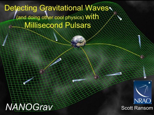
Detecting Gravitational Waves (and doing other cool physics) with ...

Detecting Gravitational Waves
(and doing other cool physics) with
Millisecond Pulsars
NANOGrav
Scott Ransom

What’s a Pulsar ?
●
●
Rotating Neutron Star!
Size of city:
– R ~ 10-20 km
●
Mass greater than Sun:
– M ~ 1.4 M sun
●
Strong Magnetic Fields:
– B ~ 10 8 -10 14 Gauss
●
●
●
Pulses are from a
“lighthouse” type effect
“Spin-down” power up to
10,000 times more than
the Sun's total output!
Weak but broadband
radio sources

High B
Pulsar Flavors
Young PSRs
(high B, fast spin,
very energetic)
Young
Normal PSRs
(average B,
slow spin)
Millisecond PSRs
(low B, very fast,
very old, very stable
spin, best for basic
physics tests)
Low B
Old

Millisecond Pulsars are Very
Precise Clocks
PSR B1937+21
At midnight on 5 Dec, 1998:
P = 1.5578064688197945 ms
+/- 0.0000000000000004 ms
The last digit changes by about 1 per second!
This extreme precision is what allows us to
use pulsars as tools to do unique physics!

How are millisecond pulsars made?
Binary system of supergiant
And a normal star
Supernova produces
a neutron star
Red Giant transfers
matter to neutron star
Millisecond Pulsar
emerges with a white
dwarf companion

Physics from Pulsars
(see Blandford, 1992, PTRSLA, 341, 177 for a review)
●
●
●
●
●
●
●
●
●
●
Newtonian and relativistic dynamics (e.g. binary pulsars)
Gravitational wave physics (e.g. binaries, MSP timing)
Physics at nuclear density (e.g. NS equations of state)
Astrophysics (e.g. stellar masses and evolution)
Plasma physics (e.g. magnetospheres, pulsar eclipses)
Fluid dynamics (e.g. supernovae collapse)
Magnetohydrodynamics (MHD; e.g. pulsar winds)
Relativistic electrodynamics (e.g. pulsar magnetospheres)
Atomic physics (e.g. NS atmospheres)
Solid state physics (e.g. NS crust properties)

Pulsar Timing
●
●
●
All of the science is
from long-term timing
Account for every
rotation of the pulsar
Fit the arrival times to
a polynomial model after transforming the time:
●
●
Accounts for pulsar spin, orbital, and astrometric
parameters and Roemer, Einstein, and Shapiro
delays in the Solar System and pulsar system
Extraordinary precision for MSP timing

Pulsar Timing
●
●
●
All of the science is
from long-term timing
Account for every
rotation of the pulsar
Fit the arrival times to
a polynomial model after transforming the time:
●
●
Accounts for pulsar spin, orbital, and astrometric
parameters and Roemer, Einstein, and Shapiro
delays in the Solar System and pulsar system
Extraordinary precision for MSP timing

Original time
series
Shift and add
the pulses
“Folding” Pulsar Data for Timing
A strong “average” profile that
can be cross correlated to
get a Time-of-Arrival (TOA)

The science is in the
residuals!:
“Good” Timing Solution
RMS precision ~ 10 -5 -10 -3 P
Position error
Uncorrected spin-down
Proper motion

Timing Sensitivity
Timing precision depends on:
– Sensitivity (A/Tsys)
– Pulse width (w)
– Pulsar flux density (S)
– Instrumentation
Jenet & Demorest 2010, in prep.

Precision Timing Example
• Astrometric Params
– RA, DEC, μ, π
• Spin Params
– P spin
, P spin
• Keplerian Orbital Params
– P orb
, x, e, ω, T 0
• Post-Keplerian Params
– ω, γ, P orb
, r , s
~100 ns RMS
timing residuals!
Recent work (e.g. Verbiest et al 2009) shows
this is sustainable over 5+ yrs for several MSPs
van Straten et al., 2001
Nature, 412, 158

Post-Keplerian Orbital Parameters
General Relativity gives:
(Advance of Periastron)
(Grav redshift + time dilation)
(Shapiro delay: “range” and “shape”)
where: T ⊙
≡ GM ⊙
/c 3 = 4.925490947 μs,
M = m 1
+ m 2
, and s ≡ sin(i)
These are only functions of:
- the (precisely!) known Keplerian orbital parameters P b
, e, asin(i)
- the mass of the pulsar m 1
and the mass of the companion m 2

The Binary Pulsar: B1913+16
●
First binary pulsar discovered at Arecibo Observatory by
Hulse and Taylor in 1974 (1975, ApJ, 195, L51)
NS-NS Binary
P psr
= 59.03 ms
P orb
= 7.752 hrs
a sin(i)/c = 2.342 lt-s
e = 0.6171
ω = 4.2 deg/yr
M c
= 1.3874(7) M ⊙
M p
= 1.4411(7) M ⊙

The Binary Pulsar: B1913+16
Three post-Keplerian Observables: ω, γ, P orb
Indirect detection of Gravitational Radiation!
From Weisberg &
Taylor, 2003

High-precision MSP Timing for
Gravitational Wave Detection
e.g. Detweiler, 1979
Hellings & Downs, 1983
●
●
The best MSPs
(timing precisions
between 50-200 ns
RMS) can be used to
search for nHz
gravitational waves
gw
~1/yrs to 1/weeks
● h ~ σ TOA
/ T ~ 10 -15
●
●
Sensitivity comparable
and complementary to
Adv. LIGO and LISA!
Need best pulsars,
instruments, and
telescopes!
Credit: D. Backer

Pulsars and GW Basics
Photon Path
k µ
Pulsar
G-wave
Earth
Flat space metric with perturbations
Frequency shifts occur along the
photon path based on the G-wave
Integral turns out to only be
based on the metric at the
Pulsar (then) and Earth (now)
Integrate over the frequency shifts
in time to get the timing residuals

So where do these GWs come from?
Coalescing Super-Massive Black Holes
•
Basically all galaxies have them
• Masses of 10 6 – 10 9 M ⊙
•
Galaxy mergers lead to BH mergers
•
When BHs within 1pc, GWs are main energy loss
• For total mass M/(1+z), distance d L
, and SMBH
orbital freq f, the induced timing residuals are:
Potentially measurable with a single MSP!

So where do these GWs come from?
3C66B
At z = 0.02
Orbital period 1.05 yrs
Total mass 5.4x10 10
(Sudou et al 2003)
10 M ⊙
Predicted timing
residuals
Ruled out by
MSP observations
Jenet et al. 2004, ApJ, 606, 799

Stochastic GW Backgrounds
An ensemble of many individual GWs, from different
directions and at different amplitudes and frequencies
Characteristic strain spectrum is (basically) a power law:
But see Sesana et al 2008
The amplitude is the only unknown for each model
e.g. Jenet et al. 2006, ApJ, 653, 1571

Best Single Pulsar Limits
Power spectrum of induced timing residuals:
Residuals (s)
PSR B1855+09
Kaspi, Taylor, Ryba. 1994, ApJ, 428, 713
Demorest 2007,
PhD Thesis

A Pulsar Timing Array (PTA)
Timing residuals due to a GW have two components:
“Pulsar components” are uncorrelated between MSPs
“Earth components” are correlated between MSPs
Signal in Residuals
Clock errors:
monopole
Ephemeris errors:
dipole
GW signal:
quadrupole
Two-point correlation function
Courtesy: G. Hobbs
e.g. Hellings & Downs, 1983, ApJL, 265, 39;
Jenet et al. 2005, ApJL, 625, 123

GW Detection with a Pulsar Timing Array
●
●
Need good MSPs and
lots of time (patience)
Significance scales
linearly with the
number of MSPs
Canonical PTA:
● Bi-weekly, multi-freq
obs for 5-10 years
● ~20-40 MSPs with
~100 ns timing RMS
● This is not easy...

NANOGrav
● About 22 members
from North America
● Observing ~20 MSPs
● Using Arecibo and the
GBT via 2 large
projects (PI Paul
Demorest)
● 2 obs freqs at GBT, 2-
3 at Arecibo per PSR
● RMS residuals from
~100ns to 1.5us
● First 4 years of data
limit h c
(1yr -1 ) < 7x10 -15
comparable to 20yrs
of single MSP
arXiv:0902.2968 and arXiv:0909.1058
http://nanograv.org

NANOGrav improvement with time...
Note complementarity
with LIGO and LISA
Courtesy P. Demorest

NANOGrav improvement with time...
Courtesy P. Demorest
Magenta and cyan curves show what happens if we
improve our ability to time the pulsars by factors of ~3 and 10

So how do we improve?
(in approx order of difficulty)
●
●
●
●
●
●
●
Patience...
International PTA
New instrumentation (more BW)
Find more and better MSPs
Better timing algorithms
Improved understanding of the systematics.
e.g. interstellar medium (ISM) effects
Bigger telescopes (i.e. FAST and SKA)

International PTA

International PTA (5yr campaign)
IPTA
NANOGrav
Courtesy J. Verbiest

GUPPI: A Pulsar “Dream Machine” for the GBT
● 800 MHz BW coherent
de-dispersion backend
● 9x more BW ~ 3x
more sensitive
● High dynamic range
(8-bit sampling) with
CASPER “iBob” with 2xADC
full polarization
boards (2Gsps each)
● Large improvement in
timing precision and
“control” of ISM effects
● “CASPER” FPGAbased
technology
from Berkeley
● Ready by end of 2009!
e.g. Parsons et al 2006;
http://seti.berkeley.edu/casper/
CASPER “BEE2” compute
board with 5 fast FPGAs

GUPPI: A Pulsar “Dream Machine” for the GBT
● 800 MHz BW coherent
de-dispersion backend
● 9x more BW ~ 3x
more sensitive
● High dynamic range
(8-bit sampling) with
CASPER “iBob” with 2xADC
full polarization
boards (2Gsps each)
● Large improvement in
timing precision and
“control” of ISM effects
● “CASPER” FPGAbased
technology
from Berkeley
● Ready by end of 2009!
e.g. Parsons et al 2006;
http://seti.berkeley.edu/casper/
CASPER “BEE2” compute
board with 5 fast FPGAs

Galactic ISM: electrons and radio waves...
• Turbulent, Ionized ISM causes
several time and radio
frequency dependent effects:
•Dispersion
•Faraday Rotation
•Multi-path propagation
•Scintillation
•Scattering
• Some effects are removable,
others aren't (yet?)...
• Much work ongoing in this area
(see recent papers by
Stinebring, Walker, Demorest,
Cordes, Shannon, Rickett etc)
From Cordes and Lazio 2001
(NE2001)

Dispersion
Lower frequency radio
waves are delayed with
respect to higher frequency
radio waves by the ionized
interstellar medium
t ∝ DM -2
(DM = Dispersion Measure)
Coherent Dedispersion
exactly removes this effect

Pulse Broadening and Scintillation
-4
Multipath causes freq dependent pulse broadening and scintillation.

More MSPs
●
●
●
●
Several large-scale searches for pulsars ongoing
around the world: (GBT, Arecibo, Parkes, Effelsberg)
MSPs are prime target: know ~1% of total in Galaxy
Many bright and high-precision MSPs have yet to be
discovered – some are very nearby
Lots of “secondary” science

PSR J1903+0327 with Arecibo P-ALFA
This thing is weird.
- Fully recycled PSR
- Highly eccentric orbit
- Massive likely mainsequence
star companion
- Massive NS (1.7 Msun)
- High precision timing
despite being distant and
in Galactic plane
Champion et al. 2008,
Science, 320, 1309
Bill Saxton, NRAO/AUI/NSF

PSR J1023+0038 is a “Missing Link” (w/ GBT)
Previously (over last 10 yrs)
detected in FIRST, optical
images/spectra, and X-rays
and identified as a strange
CV or a quiescent LMXB!
4.75 hr binary!
Evidence for accretion!
“Nasty” eclipses...
Archibald et al. 2009,
Science, 324, 1411

Very recently... Bright Fermi UnIDd Sources
Bright Radio
Binary MSPs!
Ransom et al. in prep

●
●
●
●
●
MSPs and GWs Summary
Radio pulsars can potentially directly detect
nHz frequency gravitational waves
A detection with current facilities is possible
(maybe even likely) in the next 5-15 years
– Currently limits from single pulsars and initial PTAs
are A ~ 10 -14 or slightly below (strain amplitude)
– Arecibo buys us 5 yrs, 3x more obs buys us 3 yrs
More and better MSPs for quicker detection
With future very large radio telescopes (e.g.
SKA) and many more MSPs, detailed study of
nHz GWs is likely (A ~ 10 -17 )
nanograv.org and white papers for more info

Arecibo and the IPTA

Recycled PSR Distances
The known MSPs
are local objects (and
are almost isotropically
distributed on the sky.
Gal
Center