Extracting Principal Components from Pseudo-random Data by ...

Extracting Principal Components from 

Pseudo-random Data by Using Random Matrix Theory 

Mieko Tanaka-Yamawaki 

Department of Information and Knowledge Engineering 

Graduate School of Engineering 

Tottori University, Tottori, 680-8552 Japan 

Mieko@ike.tottori-u.ac.jp 

Abstract. We develop a methodology to grasp temporal trend in a stock market 

that changes year to year, or sometimes within a year depending on numerous 

factors. For this purpose, we employ a new algorithm to extract significant 

principal components in a large dimensional space of stock time series. The key 

point of this method lies in the randomness and complexity of the stock time 

series. Here we extract significant principal components by picking a few 

distinctly large eigenvalues of cross correlation matrix of stock pairs in 

comparison to the known spectrum of corresponding random matrix derived in 

the random matrix theory (RMT). The criterion to separate signal from noise is 

the maximum value of the theoretical spectrum of We test the method using 1 

hour data extracted from NYSE-TAQ database of tickwise stock prices, as well 

as daily close price and show that the result correctly reflect the actual trend of 

the market. 

Keywords: Stock Market, Trend, Principal Component, RMT, Correlation, 

Eigenvalues. 

1 Introduction 

In a stock market, numerous stock prices move under a high level of randomness and 

some regularity. Some stocks exhibit strong correlation to other stocks. A strong 

correlation among eminent stocks should result in a visible global pattern. However, 

the networks of such correlation are unstable and the patterns are only temporal. In 

such a condition, a detailed description of the network may not be very useful, since 

the situation quickly changes and the past knowledge is no longer valid under the new 

environment. If, however, we have a methodology to extract, in a very short time, 

major components that characterize the motion of the market, it should give us a 

powerful tool to describe temporal characteristics of the market and help us to set up a 

time varying model to predict the future move of such market. 

Recently, there have been wide interest on a possible candidate for such a 

methodology using the eigenvalue spectrum of the equal-time correlation matrix 

between pairs of price time series of different stocks, in comparison to the 

corresponding matrix computed by means of random time series [1-4]. Plerau, et. al. 

[1] applied this technique on the daily close prices of stocks in NYSE and S&P500. 

R. Setchi et al. (Eds.): KES 2010, Part III, LNAI 6278, pp. 602–611, 2010. 

© Springer-Verlag Berlin Heidelberg 2010

Extracting Principal Components from Pseudo-random Data 603 

We carry on the same line of study used in Ref. [1] for the intra-day price correlations 

on American stocks to extract principal components. In this process we clarify the 

process in an explicit manner to set up our algorithm of RMT_PCM to be applied on 

intra-day price correlations. Based on this approach, we show how we track the trend 

change based on the results from year by year analysis. 

2 Cross Correlation of Price Time Series 

It is of significant importance to extract sets of correlated stock prices from a huge 

complicated network of hundreds and thousands of stocks in a market. In addition to 

the correlation between stocks of the same business sectors, there are correlations or 

anti correlations between different business sectors. 

For the sake of comparison between price time series of different magnitudes, we 

often use the profit instead of the prices [1-5]. The profit is defines as the ration of the 

increment ΔS, the difference between the price at t and t+Δt, divided by the stock 

price S(t) itself at time t. 

S(t 

+ Δt) 

− S(t) ΔS(t) 

= 

S(t) S(t) 

(1) 

This quantity does not depend on the unit, or the size, of the prices which enable us to 

deal with many time series of different magnitude. More convenient quantity, 

however, is the log-profit defined by the difference between log-prices. 

r(t) 

Since it can also be written as 

= log(S(t + Δt)) 

− log(S(t)) 

(2) 

⎛ S(t + Δt) ⎞ 

r (t) = log⎜ 

⎟ 

(3) 

⎝ S(t) ⎠ 

and the numerator in the log can be written as S(t)+ΔS(t), 

⎛ ΔS(t) 

⎞ ΔS(t) 

r(t) = log 

⎜1+ 

≅ 

S(t) 

⎟ 

(4) 

⎝ ⎠ S(t) 

It is essentially the same as the profit r(t) defined on Eq. (1). The definition in Eq.(2) 

has an advantage. 

The correlation C i,j 

between two stocks, i and j, can be written as the inner product 

of the two log-profit time series, r i (t) 

and r j (t) 

, 

T 

1 

i ,j = ∑ri 

(t)rj(t) 

T 

t= 

1 

C (5) 

We normalize each time series in order to have the zero average and the unit 

variances as follows.

604 M. Tanaka-Yamawaki 

ri 

(t) − < ri 

> 

xi(t) 

= (i=1,…,N) (6) 

σi 

Here the suffix i indicates the time series on the i-th member of the total N stocks. 

The correlations defined in Eq. (5) makes a square matrix whose elements are in 

general smaller than one. 

| j 

Ci, 

| ≤ 1 (i=1,…,N; j=1,…,N) (7) 

and its diagonal elements are all equal to one due to normalization. 

C i , i = 1 (i=1,…,N) (8) 

Moreover, it is symmetric 

C i,j 

= C j,i 

(i=1,…,N; j=1,…,N) (9) 

As is well known, a real symmetric matrix C can be diagonalized by a similarity 

transformation V -1 CV by an orthogonal matrix V satisfying V t =V -1 , each column of 

which consists of the eigenvectors of C. 

Such that 

⎛ vk,1 

⎞ 

⎜ ⎟ 

⎜ vk,2 

⎟ 

v k = ⎜ ⎟ 

(10) 

. 

⎜ ⎟ 

⎝ vk,N 

⎠ 

C v k = λ v (k=1,…,N) (11) 

k 

k 

where the coefficient λ k 

is the k-th eigenvalue. 

Eq.(11) can also be written explicitly by using the components as follows. 

N 

∑C 

j= 

1 

v 

i, 

j k, j 

= λ 

k 

v 

k,i 

(12) 

The eigenvectors in Eq.(10) form an ortho-normal set. Namely, each eigenvector 

v is normalized to the unit length 

k 

v 

N 

2 

k ⋅ vk 

= ∑ (vk,n 

) = 

n= 

1 

and the vectors of different suffices k and l are orthogonal to each other. 

1 

(13) 

v 

N 

k ⋅ vl 

= ∑ vk,nvl,n 

= 

n= 

1 

Equivalently, it can also be written as follows by using Kronecker’s delta. 

0 

(14)


v 

⋅ = δ 

(15) 

k v l 

k,l 

The right hand side of Eq.(15) is zero(one) for k ≠ l(k = l) 

. The numerical solution of 

the eigenvalue problem of a real symmetric matrix can easily be obtained by repeating 

Jacobi rotations until all the off-diagonal elements become close enough to zero. 

3 RMT-Oriented Principal Component Method 

The diagonalization process of the correlation matrix C by repeating the Jacobi 

rotation is equivalent to convert the set of the normalized set of time series in Eq. (6) 

into the set of eigenvectors. 

⎛ x1(t) 

⎞ 

⎜ ⎟ 

⎜ . ⎟ 

y(t) = ( V) ⎜ . ⎟ = Vx(t) 

(16) 

⎜ ⎟ 

⎜ . ⎟ 

⎜ ⎟ 

⎝ x N (t) ⎠ 

It can be written explicitly using the components as follows. 

N 

y (t) = ∑ v 

i 

j= 

1 

i, j 

x 

j 

(t) 

(17) 

The eigenvalues can be interpreted as the variance of the new variable discovered by 

means of rotation toward components having large variances among N independent 

variables. Namely, 

σ 

= 

2 

1 

T 

N 

i 

1 

T 

T 

N 

N 

T 

t= 

1 

∑∑v 

i,l 

t= 1l 

= 1 

= ∑∑v 

∑(y 

i,l 

l= 1m= 

1 

= λ 

= 

v 

i 

(t)) 

l 

i,m 

C 

2 

N 

x (t) ∑ v 

i,m 

m= 

1 

l,m 

x 

m 

(t) 

(18) 

Since the average of y i 

over t is always zero based on Eq.(6) and Eq.(17). For the 

sake of simplicity, we name the eigenvalues in discending order, λ 1 > λ2 

> ... > λN 

. 

The theoretical base underlying the principal component analysis is the expectation 

of distinguished magnitudes of the principal components compared to the other 

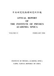
components in the N dimensional space. We illustrate in Fig.1 the case of 2 

dimensional data (x,y) rotated to a new axis z=ax+by and w perpendicular to z, in 

which z being the principal component and this set of data can be described as 1 

dimensional information along this principal axis.


y 

z 

x 

Fig. 1. A set of four 2-dimensional data points are characterized as a set of 1-dimensional data 

along z axis 

If the magnitude of the largest eigenvalue λ 1 of C is significantly large compared 

to the second largest eigenvalue, then the data are scattered mainly along this 

principal axis, corresponding to the direction of the eigenvector v 1 of the largest 

eigenvalue. This is the first principal component. Likewise, the second principal 

component can be identified to the eigenvector v 2 of the second largest eigenvalue 

perpendicular to v 1 . Accordingly, the 3 rd and the 4 th principal components can be 

identified as long as the components toward these directions have significant 

magnitude. The question is how many principal components are to be identified out of 

N possible axes. 

One criterion is to pick up the eigenvalues larger than 1. The reason behind this 

scenario is the conservation of trace, the sum of the diagonal elements of the matrix, 

under the similarity transformation. Due to Eq. (8), we obtain 

N 

∑λ k = N 

k= 

1 

which means there exists m such that λk > 1 for k < k m 

, and λ k < 1 for k > k m 

. As was 

shown in Re1.[1], this criterion is too loose to use for the case of the stock market 

having N > 400. There are several hundred eigenvalues that are larger than 1, and 

many of the corresponding eigenvector components are literally random and do not 

carry useful information. 

Another criterion is to rely on the accumulated contribution. It is recommended by 

some references to regard the top 80% of the accumulated contribution are to be 

regarded as the meaningful principal components. This criterion is too loose for the 

stock market of N > 400, for m easily exceeds a few hundred. 

A new criterion proposed in Ref. [1-4] and examined recently in many real stock 

data is to compare the result to the formula derived in the random matrix theory [6]. 

According to the random matrix theory (RMT, hereafter), the eigenvalue distribution 

spectrum of C made of random time series is given by the following formula[7] 

( λ+ − λ)( 

λ − λ−) 

P ( λ) 

= Q 

RMT 

(20) 

2π 

λ 

in the limit of N → ∞, T → ∞, 

Q = T / N = const. 

(19)


where T is the length of the time series and N is the total number of independent time 

series (i.e. the number of stocks considered). This means that the eigenvalues of 

correlation matrix C between N normalized time series of length T distribute in the 

following range. 

λ − < λ < λ + 

(21) 

Following the formula Eq. (19), between the upper bound and the lower bound given 

by the following formula. 

1 1 

λ ± = 1 + ± 2 

(22) 

Q Q 

The proposed criterion in our RMT_PCM is to use the components whose 

eigenvalues, or the variance, are larger than the upper bound given by RMT. 

λ + 

λ >> λ (23) 

+ 

4 Cross Correlation of Intra-day Stock Prices 

In this chapter we report the result of applying the method of RMT_PCM on intra-day 

stock prices. The data sets we used are the tick-wise trade data (NYSE-TAQ) for the 

years of 1994-2002. We used price data for each year to be one set. In this paper we 

mention our result on 1994, 1998 and 2002. 

One problem in tickdata is the lack of regularity in the traded times. We have 

extracted N stocks out of all the tick prices of American stocks each year that have at 

least one transaction at every hour of the days between 10 am to 3 pm. This provides 

us a set of price data of N symbols of stocks with length T, for each year. For 1994, 

1998 and 2002, the number of stock symbols N as 419, 490, and 569, respectively. 

The length of data T was 1512, six (per day) times 252, the number of working days 

of the stock market in the above three years. 

The stock prices thus obtained becomes a rectangular matrix of S i,k where i=1,…,N 

represents the stock symbol and k=1,…, T represents the executed time of the stock. 

The i-th row of this price matrix corresponds to the price time series of the i-th 

stock symbol, and the k-th column corresponds to the prices of N stocks at the time k. 

We summarize the algorithm that we used for extracting significant principal 

components from 1 hour price matrix in Table 1. 

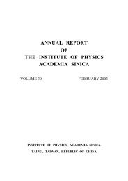
Following the procedure described so far, we obtain the distribution of eigenvalues 

shown in Fig. 2 for the 1-hour stock prices for N = 419 and T = 1512 in 1994. 

The histogram shows the eigenvalues (except the largest λ 1 = 46.3), λ 2 = 5.3, λ 3 = 

5.1, λ 4 = 3.9, λ 5 = 3.5, λ 6 = 3.4, λ 7 = 3.1, λ 8 = 2.9, λ 9 = 2.8, λ 10 = 2.7 λ 11 = 2.6, 

λ 12 = 2.6, λ 13 = 2.6 λ 14 = 2.5 λ 15 = 2.4, λ 16 = 2.4 λ 17 = 2.4 and the bulk distribution of 

eigenvalues under the theoretical maximum,λ + = 2.3. These are compared with the 

RMT curve of Eq. (20) for Q = 1512 / 419 =3.6.


Table 1. The algorithm to extract the significant principal components (RMT_PCM) 

Algorithm of RMT_PCM: 

1. Select N stock symbols for which the traded price exist for all 

t=1,,T. (6 times a day, at every hour from 10 am to 3 pm, on every 

working day of the year). 

2. Compute log-return r(t) for all the stocks. Normalize the time series 

to have mean=0, variance=0, for each stock symbol, i=1,, N. 

3. Compute the cross correlation matrix C and obtain eigenvalues and 

eigenvectors 

4. Select eigenvalues larger than 

in Eq.(22), the upper limit of the 

RMT spectrum, Eq. (20). 

Probability density P(λ) 

1.2 

0.8 

0.4 

Probability density P(λ) 

1994-1h 

RMT 419-1512 

0.1 

0.08 

λ1 = 46.3 

0.04 

0 

0 20 40 50 

Eigenvalue λ 

0 

0 1 2 3 4 5 6 

Eigenvalue λ 

Fig. 2. Distribution of eigenvalues of correlation matrix of N=419 stocks for T=1512 data in 

1994 compared to the corresponding RMT in Eq. (20) for Q= T/N =3.6 

Corresponding result of 1998 data gives, for N=490, T=1512, there are 24 

eigenvalues: λ 1 =81.12,λ 2 =10.4 λ 3 = 6.9 λ 4 = 5.7, λ 5 = 4.8, λ 6 = 3.9, λ 7 = 3.5, λ 8 = 3.5, 

λ 9 = 3.4, λ 10 = 3.2, λ 11 = 3.1,λ 12 = 3.1, λ 1 3 = 3.0,λ 14 = 2.9, λ 15 = 2.9,λ 16 = 2.8, λ 17 = 2.8, 

λ 18 = 2.8, λ 19 = 2.7, λ 20 = 2.7, λ 21 = 2.6,λ 22 = 2.6, λ 23 = 2.5,λ 24 = 2.5 and the bulk 

distribution of eigenvalues under the theoretical maximum, λ + = 2.46. These are 

compared with the RMT curve of Eq. (20) for Q = 1512 / 490 = 3.09. 

Similarly, we obtain for 2002 data, for N=569, T=1512, there are 19 eigenvalues, 

λ 1 = 166.6, λ 2 = 20.6, λ 3 = 11.3, λ 4 = 8.6, λ 5 = 7.7, λ 6 = 6.5, λ 7 = 5.8, λ 8 = 5.3, λ 9 = 

4.1, λ 10 =4.0,λ 11 = 3.8, λ 12 = 3.5,λ 13 = 3.4, λ 14 = 3.3,λ 15 = 3.0,λ 16 = 3.0,λ 17 = 2.9, λ 18 = 

2.8= 3.0,λ 19 = 2.6, and the bulk distribution under the theoretical maximum, λ + = 

2.61. These are compared with the RMT curve of Eq. (12) for Q = 1512 / 569 = 2.66.


However, a detailed analysis of the eigenvector components tells us that the 

random components are not necessarily reside below the upper limit of RMT, λ + , but 

percolates beyond the RMT limit if the sequence is not perfectly random. Thus it is 

more reasonable to assume that the border between the signal and the noise is 

somewhat larger than λ + . This interpretation also explains the fact that the eigenvalue 

spectra always spreads beyond λ + . It seems there is no more mathematical reason to 

decide the border between signal and noise. We return to data analysis in order to 

obtain further insight for extracting principal components of stock correlation. 

5 Eigenvectors as the Principal Components 

The eigenvector v 1 corresponding to the largest eigenvalue is the 1 st principal 

component. For 1-hour data of 1994 where we have N=419 and T=1512, the major 

components of U 1 are giant companies such as GM, Chrysler, JP Morgan, Merrill 

Lynch, and DOW Chemical. The 2 nd principal component v 2 consists of mining 

companies, while the 3 rd principal component v 3 consists of semiconductor 

manufacturers, including Intel. The 4 th principal component v 4 consists of computer 

and semiconductor manufacturers, including IBM, and the 5 th component v 5 consists 

of oil companies. The 6 th and later components do not have distinct features compared 

to the first 5 components and can be regarded as random. 

For 1-hour data of 1998 where we have N=490 and T=1512, the major components 

of v 1 are made of banks and financial services. The 2 nd principal component v 2 

consists of 10 electric companies, while v 3 consists of banks and financial services, 

and U 4 consists of semiconductor manufacturers. The 6 th and later components do not 

have distinct features compared to the first 5 components and regarded as random. 

For 1-hour data of 2002 where we have N=569 and T=1512, the major components 

of v 1 are strongly dominated by banks and financial services, while v 2 are strongly 

dominated by electric power supplying companies, which were not particularly visible 

in 1994 and 1998. 

The above observation summarized in Table 2 indicates that Appliances/Car and 

IT dominated the industrial sector in 1994, which have moved toward the dominance 

of Finance, Food, and Electric Power Supply in 2002. 

Table 2. Business sectors of top 10 components of 5 principal components in 1994, 1998 and 

2002 

v k 1994 1998 2002 

v 1 Finance(4), IT(2), Finance(8) Finance(9) 

Appliances/Car(3) 

v 2 Mining(7), Finance(2) Electric(10) Food(6) 

v 3 IT (10) Finance(3) Electric(10) 

v 4 IT(7),Drug(2) IT (10) Food(4), Finance(2),Electric (4) 

v 5 Oil(9) Mining(6) Electric (9)


6 Separation of Signal from Noize 

Although this method works quite well for v 1 - v 5 ,the maximum eigenvalueλ + seems 

too loose to be used for a criterion to separate signal from the noise. There are many 

eigenvalues near λ + which are practically random. In Fig.2, for example, only the largest 

five eigenvalues exhibit distinct signals and the rest can be regarded more or less 

random components. In this respect, we examine the validity of RMT for finite values 

of N and T. Is there any range of Q under which the RMT formula breaks down? 

First of all, we examine how small N and T can be. We need to know whether 

N=419-569 and T=1512 in our study in this paper are in any adequate range. To do 

this, we use two kinds of computer-generated random numbers, the random numbers 

of normal distribution generated by Box-Muller formula, and the random numbers of 

uniform distribution generated by the rand( ) function. However, if we shuffle the 

generated numbers to increase randomness, the eigenvalue spectra perfectly match the 

RMT formula. 

The above lesson tells us that the machine-generated random numbers, 

independent of their statistical distributions, such as uniform or Gaussian, become a 

set of good random numbers only after shuffling. Without shuffling, the random 

series are not completely random according to the sequence, while the evenness of 

generated numbers is guaranteed. 

Taking this in mind, we test how the formula in Eq.(20) works for various values 

of parameter N and Q. Our preliminary result shows that the errors are negligible in 

the entire range of N > 50 for T > 50 (Q > 1), after shuffling. 

7 Summary 

In this paper, we propose a new algorithm RMT-oriented PCM and examined its 

validity and effectiveness by using the real stock data of 1-hour price time series 

extracted from the tick-wise stock data of NYSE-TAQ database of 1994, 1998, and 

2002. We have shown that this method provides us a handy tool to compute the 

principal components v 1 - v 5 in a reasonably simple procedure. 

We have also tested the method by using two different machine-generated random 

numbers and have shown that those random numbers work well for a wide range of 

parameters, N and Q, only if we shuffle to randomize the machine-generated random 

series. 

References 

1. Plerou, V., Gopikrishnan, P., Rosenow, B., Amaral, L.A.N., Stanley, H.E.: Random matrix 

approach to cross correlation in financial data. Physical Review E, American Institute of 

Physics 65, 66126 (2002) 

2. Plerou, V., Gopikrishnan, P., Rosenow, B., Amaral, L.A.N., Stanley, H.E.: Physical Review 

Letters. American Institute of Physics 83, 1471–1474 (1999) 

3. Laloux, L., Cizeaux, P., Bouchaud, J.-P., Potters, M.: American Institute of Physics, vol. 83, 

pp. 1467–1470 (1999)


4. Bouchaud, J.-P., Potters, M.: Theory of Financial Risks. Cambridge University Press, 

Cambridge (2000) 

5. Mantegna, R.N., Stanley, H.E.: An Introduction to Econophysics: Correlations and 

Complexity in Finance. Cambridge University Press, Cambridge (2000) 

6. Mehta, M.L.: Random Matrices, 3rd edn. Academic Press, London (2004) 

7. Sengupta, A.M., Mitra, P.P.: Distribution of singular values for some random matrices. 

Physical Review E 60, 3389 (1999)

Extracting Principal Components from Pseudo-random Data by ...

You also want an ePaper? Increase the reach of your titles

Delete template?

Save as template?