1. Phase portrait for the damped pendulum
1. Phase portrait for the damped pendulum
1. Phase portrait for the damped pendulum

Create successful ePaper yourself
Turn your PDF publications into a flip-book with our unique Google optimized e-Paper software.
2/3/2013 1<br />
PHY 380.03, Fall 2010 Homework 2 Solution<br />
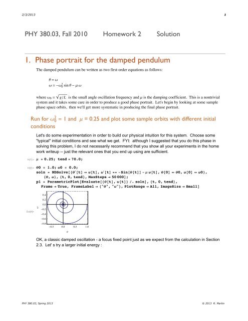
<strong>1.</strong> <strong>Phase</strong> <strong>portrait</strong> <strong>for</strong> <strong>the</strong> <strong>damped</strong> <strong>pendulum</strong><br />
The <strong>damped</strong> <strong>pendulum</strong> can be written as two first-order equations as follows:<br />
q = w<br />
w = -w 0 2 sin q - m w<br />
where w 0 = gêL is <strong>the</strong> small angle oscillation frequency and m is <strong>the</strong> damping coefficient. This is a nontrivial<br />
system and it takes some care in order to produce a good phase <strong>portrait</strong>. Let's begin by looking at some sample<br />
phase space orbits, <strong>the</strong>n we'll get more systematic in producing <strong>the</strong> final phase <strong>portrait</strong>.<br />
Run <strong>for</strong> w 0 2 = 1 and m = 0.25 and plot some sample orbits with different initial<br />
conditions<br />
Let's do some experimentation in order to build our physical intuition <strong>for</strong> this system. Choose some<br />
"typical" initial conditions and see what we get. FYI: although I suggested that you do this phase in<br />
solving this problem, I do not necessarily recommend that you show all your experiments in <strong>the</strong> home<br />
work writeup -- just <strong>the</strong> relevant ones that you end up using are sufficient.<br />
In[1]:= m = 0.25; tend = 70.0;<br />
In[2]:= q0 = <strong>1.</strong>0; w0 = 0.0;<br />
soln = NDSolve@8q £ @tD ã w@tD, w £ @tD == -Sin@q@tDD - m w@tD, q@0D ã q0, w@0D ã w0
2/3/2013 2<br />
In[5]:= q0 = 3; w0 = 0.0;<br />
soln = NDSolve@8q £ @tD ã w@tD, w £ @tD == -Sin@q@tDD - m w@tD, q@0D ã q0, w@0D ã w0
2/3/2013 3<br />
In[13]:= q0 = 15.0; w0 = -2.0;<br />
soln = NDSolve@8q £ @tD ã w@tD, w £ @tD == -Sin@q@tDD - m w@tD, q@0D ã q0, w@0D ã w0
What do you see here? For clarity, I left off <strong>the</strong> first orbit since it just adds confusion near <strong>the</strong> origin fixed point. I<br />
hope what's happening is becoming clear: all orbits end up attracted to one of <strong>the</strong> many stable fixed points at even<br />
multiples of p. Which one <strong>the</strong>y end up attracted to depends on <strong>the</strong>ir initial conditions. It turns out that <strong>for</strong> any<br />
attracting set, <strong>the</strong>re is a region of initial conditions attracted to it, meaning that all initial conditions in that region<br />
are attracted to <strong>the</strong> same attracting set. The attracting set <strong>for</strong> a particular attractor is called its basin of attraction.<br />
2/3/2013 4<br />
The attracting sets here are <strong>the</strong> attracting fixed points. So our goal now, in order to produce a meaningful phase<br />
<strong>portrait</strong>, is to depict <strong>the</strong> basins of attraction <strong>for</strong> each attracting fixed point. The boundaries of <strong>the</strong> attracting basins<br />
are orbits that separate basins - as it turns out, <strong>the</strong> basin boundaries will be what was <strong>the</strong> separatrix in <strong>the</strong><br />
un<strong>damped</strong> <strong>pendulum</strong>. Given this and <strong>the</strong> plot above it's a good guess that <strong>the</strong> basin boundaries are connected to<br />
<strong>the</strong> unstable hyperbolic fixed points at odd multiples of p. This basin boundary is not easy to plot since, as in <strong>the</strong><br />
dissipationless <strong>pendulum</strong>, it represents an idealized orbit. We can explore near <strong>the</strong> hyperbolic fixed point at q ã p<br />
to get a sense if what's happening. Let's see if we can determine <strong>the</strong>se basin boundaries approximately by plotting<br />
<strong>for</strong>ward and backward in time.<br />
Let's look at initial conditions very close to p: here's one that's equal to p to 6 significant digits, but slightly smaller<br />
than p:<br />
In[20]:= fp1 = 0.0; q0 = fp1 + 3.141592; w0 = 0.0;<br />
soln = NDSolve@8q £ @tD ã w@tD, w £ @tD == -Sin@q@tDD - m w@tD, q@0D ã q0, w@0D ã w0
2/3/2013 5<br />
A couple things to notice: (1) <strong>the</strong> orbits never cross, but <strong>the</strong>y intertwine, and (2) we get a hint of <strong>the</strong> old "football"<br />
shaped separatrix from <strong>the</strong> un<strong>damped</strong> <strong>pendulum</strong>, but only in <strong>the</strong> upper left and lower right quadrants. One way to<br />
remedy <strong>the</strong> second point is to integrate <strong>the</strong> equation of motion backwards in time -- in o<strong>the</strong>r words, use a negative<br />
end time:<br />
In[25]:= q0 = fp1 + 3.141592; w0 = 0.0;<br />
soln = NDSolve@8q £ @tD ã w@tD, w £ @tD == -Sin@q@tDD - m w@tD, q@0D ã q0, w@0D ã w0
2/3/2013 6<br />
In[30]:= q0 = fp1 - 3.141592; w0 = 0.02;<br />
soln = NDSolve@8q £ @tD ã w@tD, w £ @tD == -Sin@q@tDD - m w@tD, q@0D ã q0, w@0D ã w0
2/3/2013 7<br />
In[37]:= q0 = fp1 - 3.141592; w0 = 0.0;<br />
soln = NDSolve@8q £ @tD ã w@tD, w £ @tD == -Sin@q@tDD - m w@tD, q@0D ã q0, w@0D ã w0
2/3/2013 8<br />
In[48]:= fp1 = -2 p; q0 = fp1 + 3.141592; w0 = 0.0;<br />
soln = NDSolve@8q £ @tD ã w@tD, w £ @tD == -Sin@q@tDD - m w@tD, q@0D ã q0, w@0D ã w0
2/3/2013 9<br />
In[60]:=<br />
All3 = ShowAp7, p8, p9, p10, p11, p12, pl1,<br />
pl2, pl3, pl4, pl5, pl6, plo1, plo2, plo3, plo4, plo5, plo6,<br />
PlotRange Ø 88-6 p, 6 p
2/3/2013 10<br />
Put it all toge<strong>the</strong>r and you have a pretty good picture of <strong>the</strong> dynamics of a <strong>damped</strong> <strong>pendulum</strong>! Note that<br />
I've left some whitespace in <strong>the</strong> upper right and lower left corners of <strong>the</strong> plot. We could have written<br />
some code to repeat all <strong>the</strong> relevant orbits <strong>for</strong> <strong>the</strong> four remaining attracting fixed point on this plot but,<br />
by symmetry, <strong>the</strong> results will be identical to <strong>the</strong> three basins show here shifted to each new fixed point.<br />
In[96]:=<br />
Show@All3, plo7, plo8, plo9, plo10, plo11, plo12,<br />
PlotLabel Ø "<strong>Phase</strong> <strong>portrait</strong> <strong>for</strong> <strong>damped</strong> <strong>pendulum</strong>", ImageSize Ø LargeD<br />
<strong>Phase</strong> <strong>portrait</strong> <strong>for</strong> <strong>damped</strong> <strong>pendulum</strong><br />
4<br />
2<br />
Out[96]=<br />
q °<br />
0<br />
-2<br />
-4<br />
-6 p -4 p -2 p 0 2 p 4 p 6 p<br />
q<br />
This is a pretty good portrayal of <strong>the</strong> <strong>damped</strong> <strong>pendulum</strong>. You see 2 orbits within each of <strong>the</strong> three basins of<br />
attraction, one starting at positive and one at negative angular velocity (green orbits). Depending on <strong>the</strong> initial<br />
condition on each of <strong>the</strong>se orbits <strong>the</strong>y could represent: (1) a rotation that damps down into an oscillation and<br />
eventually to no motion (high initial velocity), or (2) an oscillation that damps down to no motion (low initial<br />
velocity).<br />
In class we showed that <strong>the</strong>re should be stable focus fixed points at even multiples of q = p and unstable hyperbolic<br />
points at odd multiples of q = p (all at q ° = 0). That is clearly correct looking at <strong>the</strong> plot.<br />
2. Fixed points of four nonlinear oscillators<br />
We consider three nonlinear oscillators and find three fixed points. You were asked to choose one and determine<br />
<strong>the</strong> type and stability of <strong>the</strong> fixed points. Here, I'll do all three.<br />
A. The <strong>damped</strong> Duffing oscillator<br />
The equation of motion is x – + m x ° + w 0 2 x + e x 3 = 0 and <strong>the</strong> fixed points are given by setting x ° = x – = 0,<br />
leaving<br />
xIw 0 2 + e x 2 M = 0,<br />
which gives three values of x at <strong>the</strong> fixed points: x * = 0, ±Â w 0 í<br />
e . The imaginary values cannot<br />
represent physically meaningful positions so <strong>the</strong>re is only real fixed point in phase space:<br />
PHY 380.03, Spring 2013<br />
Hx 1 * , v 1 * L = H0, 0L<br />
© 2013 R. Martin
leaving<br />
xIw 0 2 + e x 2 M = 0,<br />
2/3/2013 11<br />
which gives three values of x at <strong>the</strong> fixed points: x * = 0, ±Â w 0 í e . The imaginary values cannot<br />
represent physically meaningful positions so <strong>the</strong>re is only real fixed point in phase space:<br />
Hx 1 * , v 1 * L = H0, 0L<br />
B. The Lotka-Volterra equations<br />
The equations of motion are already in standard <strong>for</strong>m:<br />
x ° = Hb - p yL x = F x Hx, yL<br />
y ° = Hr x - dL y = F y Hx, yL<br />
and <strong>the</strong> fixed points are given by setting x ° = y ° = 0, leaving<br />
xHb - p yL = 0 and yHr x - dL = 0,<br />
From <strong>the</strong> first equation we have ei<strong>the</strong>r x = 0 or y = bêp and from <strong>the</strong> second equation we have ei<strong>the</strong>r<br />
y = 0 or x = d êr. Combining, we have two possible fixed points:<br />
Hx 1 * , v 1 * L = H0, 0L<br />
Hx 2 * , v 2 * L = Hd êr, bêpL<br />
If x and y represent <strong>the</strong> numbers of predator and prey species, <strong>the</strong> first fixed point represents both<br />
populations dying out, while <strong>the</strong> second fixed point represents an equilibrium value of <strong>the</strong> populations.<br />
C. The Rayleigh Oscillator<br />
The equation of motion is x – + eJx ° 2 - 1N x ° + x = 0 and <strong>the</strong> fixed points are given by setting x ° = x – = 0 <strong>the</strong><br />
first two terms vanish, leaving<br />
x = 0,<br />
which gives one value of x at <strong>the</strong> fixed points, so <strong>the</strong>re is one fixed point at <strong>the</strong> origin in phase space:<br />
Hx 1 * , v 1 * L = H0, 0L<br />
D. Van der Pol oscillator<br />
This equation of motion is x – - eI1 - x 2 M x ° + x = 0 and <strong>the</strong> fixed points are given by setting x ° = x – = 0, again<br />
leaves only<br />
x = 0,<br />
which is <strong>the</strong> same as <strong>the</strong> Rayleigh oscillator and gives one value of x at <strong>the</strong> fixed points, so <strong>the</strong>re is one<br />
fixed point at <strong>the</strong> origin:<br />
PHY 380.03, Spring 2013<br />
Hx 1 * , v 1 * L = H0, 0L<br />
© 2013 R. Martin
This equation of motion is x - eI1 - x M x + x = 0 and <strong>the</strong> fixed points are given by setting x = x = 0, again<br />
leaves only<br />
2/3/2013 12<br />
x = 0,<br />
which is <strong>the</strong> same as <strong>the</strong> Rayleigh oscillator and gives one value of x at <strong>the</strong> fixed points, so <strong>the</strong>re is one<br />
fixed point at <strong>the</strong> origin:<br />
Hx 1 * , v 1 * L = H0, 0L<br />
Problem 3: Stability of Rayleigh fixed points<br />
I'll apply <strong>the</strong> methods discussed in class, ei<strong>the</strong>r <strong>the</strong> stability matrix or, <strong>for</strong> Newtonian systems, all you<br />
have to do is compute <strong>the</strong> two coefficients a and b of <strong>the</strong> linearized equation(s) of motion.<br />
The equation of motion is x – + eJx ° 2 - 1N x ° + x = 0 and <strong>the</strong> only fixed point is:<br />
Hx 1 * , v 1 * L = H0, 0L<br />
This is a Newtonian system, with FHx, vL = -eIv 2 - 1M v - x so we use <strong>the</strong> standard method from class.<br />
The linear coefficients are:<br />
a = ∂F ∂F<br />
= -1, and b = = ∂x H0,0L ∂v H0,0L -IeIv2 - 1M + 2 e v 2 M = e<br />
H0,0L<br />
Here <strong>the</strong> coefficient a is always negative, while b depends on <strong>the</strong> value of e. The discriminant is<br />
b 2 + 4 a = e 2 - 4. If e 2 > 4, both eigenvalues will be real and positive, while if <strong>the</strong> opposite is true <strong>the</strong><br />
eigenvalues will be complex with a positive real part. By <strong>the</strong> results of our general 2-D fixed point<br />
derivation in class, this means <strong>the</strong> fixed point is ei<strong>the</strong>r a focus or a node. Since e > 0, <strong>the</strong> fixed point is<br />
unstable, so this fixed point is:<br />
an unstable node if e 2 > 4 and e > 0<br />
an unstable star/improper node if e 2 = 4 and e > 0<br />
an unstable focus if e 2 < 4 and e > 0<br />
Here, if we increase e from less than 2 to greater than 2, <strong>the</strong>re will be a bifurcation at e = 2 as <strong>the</strong> fixed<br />
point changes from a focus to a node.<br />
Note that you can also use <strong>the</strong> stability matrix:<br />
M = 0 1<br />
a b<br />
and <strong>the</strong> eigenvalues are given by<br />
det<br />
-a 1<br />
a<br />
b - a<br />
= a 2 - b a - a = 0<br />
with a = -1 and b = e <strong>the</strong> solution is<br />
PHY 380.03, Spring 2013<br />
a = e± e2 -4<br />
2<br />
which yields to same fixed point character as <strong>the</strong> calculation above (of course).<br />
© 2013 R. Martin
-a 1<br />
det<br />
= a 2 - b a - a = 0<br />
a b - a<br />
2/3/2013 13<br />
with a = -1 and b = e <strong>the</strong> solution is<br />
a = e± e2 -4<br />
2<br />
which yields to same fixed point character as <strong>the</strong> calculation above (of course).<br />
PHY 380.03, Spring 2013<br />
© 2013 R. Martin