Kater Pendulum

Objectives
Kater Pendulum
o To make a precision measurement of the local acceleration due to gravity
o To consider the propagation of errors in such an experiment
o To learn about computer interfacing
Reading Assignment
o Class Website – readings for this experiment
Introduction
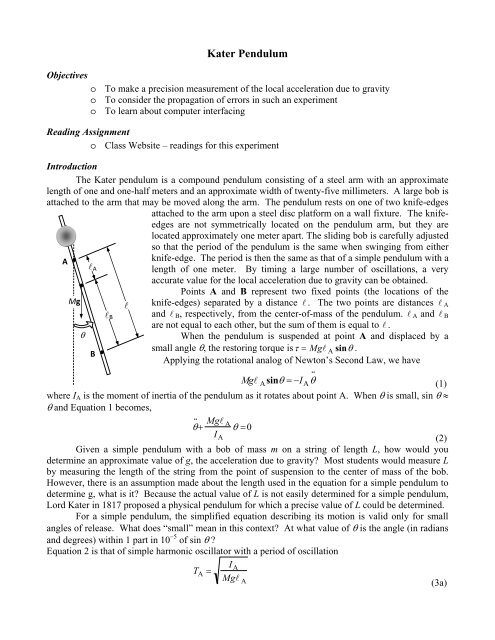
The Kater pendulum is a compound pendulum consisting of a steel arm with an approximate
length of one and one-half meters and an approximate width of twenty-five millimeters. A large bob is
attached to the arm that may be moved along the arm. The pendulum rests on one of two knife-edges
attached to the arm upon a steel disc platform on a wall fixture. The knifeedges
are not symmetrically located on the pendulum arm, but they are
located approximately one meter apart. The sliding bob is carefully adjusted
so that the period of the pendulum is the same when swinging from either
A
knife-edge. The period is then the same as that of a simple pendulum with a
lA
length of one meter. By timing a large number of oscillations, a very
accurate value for the local acceleration due to gravity can be obtained.
Points A and B represent two fixed points (the locations of the
Mg
l knife-edges) separated by a distance l . The two points are distances l A
l B and l B , respectively, from the center-of-mass of the pendulum. l A and l B
are not equal to each other, but the sum of them is equal to l .
θ
When the pendulum is suspended at point A and displaced by a
small angle θ, the restoring torque is τ = Mgl A sinθ .
B
Applying the rotational analog of Newton’s Second Law, we have
Mgl A sinθ =−I A θ
(1)
where I A is the moment of inertia of the pendulum as it rotates about point A. When θ is small, sin θ ≈
θ and Equation 1 becomes,
..
θ+ Mgl A
θ =0
I A (2)
Given a simple pendulum with a bob of mass m on a string of length L, how would you
determine an approximate value of g, the acceleration due to gravity? Most students would measure L
by measuring the length of the string from the point of suspension to the center of mass of the bob.
However, there is an assumption made about the length used in the equation for a simple pendulum to
determine g, what is it? Because the actual value of L is not easily determined for a simple pendulum,
Lord Kater in 1817 proposed a physical pendulum for which a precise value of L could be determined.
For a simple pendulum, the simplified equation describing its motion is valid only for small
angles of release. What does “small” mean in this context? At what value of θ is the angle (in radians
and degrees) within 1 part in 10 −5 of sin θ ?
Equation 2 is that of simple harmonic oscillator with a period of oscillation
..
T A =
I A
Mgl A
(3a)

Similarly, if the pendulum is suspended at point B, the period is given by
I B
T B =
Mgl B
(3b)
By applying the parallel axis theorem, we can write
2
2
I A = I CM + Ml A and I B = I CM + Ml B (4)
where I CM is the moment of inertia of the pendulum about the center-of-mass. Then, substitute
equations 4 into equations 3a and 3b and assume that the system has been arranged so that periods T A
and T B are equal. With this assumption, equations 3a and 3b are set equal to each other and I CM can be
determined.
I CM = Ml A l B (5)
Substituting this result into either equation 3a or 3b gives
T = T A = T B = 2π
or
l A +l B
g
T = 2π
l g
(6)
Our goal is to measure g to a precision in the range 10 –4 to 10 –5 . Measuring g with precision
and accuracy requires that the period and the length between the two pivot points be determined with
precision and accuracy. Since the standard error of the mean value, a measure of how well we know
the average of multiple measurements is the true value, is given by
s
σ x
=
N
(7)
where s is the standard deviation and N is the number of measurements. From past experience, the
deviation between successive measurements is on the order of 10 –4 , so if we want to increase our
precision by a factor of ten, we must make at least 100 measurements of the period.
Experimental Procedure
Part A: Preparation of the Kater Pendulum
Familiarize yourself with the Kater pendulum and its fixture. Note: the knife edge rests on a
metal platform that can be damaged by dropping the pendulum onto it. Each time the
pendulum is to be replaced on the platform, the pendulum must be gently lowered onto it so as
not to damage it.
Note the markings on the thin side that may be used to measure the position of the bob.
Position the bob so that it is at the zero position (the line closest to the knife edge). Carefully
and gently return the pendulum to the wall fixture. Failure to gently set the knife edge on the
platform will result in damage to the platform, which produces a very large error.

Part B: Knife-edge separation distance
1. The distance between the knife edges is measured using a good precision cathetometer with
a range of one meter. Set up the cathetometer and become familiar with its use.
2. Each student in the group should take a turn at measuring l , the distance between the two
knife-edges. Record each measurement separately and independently. When everyone has
made the measurement, then each student should record the other students’ measurements.
The group will then determine and average value of l to use in the calculation of g.
Part C: Period timing
1. A photogate is used to measure the period as the pendulum swings. Set up the photogate so
that it is fixed in place at the lowest position of the pendulum swing.
2. A small angle of release is required by the theory for this experiment. As a group,
determine a value for the small angle that will be consistently used for all measurements
during the experiment. Use the protractor provided. For all measurements, the same
release position will be used. Be sure to write down the results of your group discussion on
this issue in your notebook.
3. The Data Studio computer program has been set up to have a 30 second delay before data is
collected and stored. This is designed to minimize effects due to a wobble introduced when
the pendulum is released. Very gently release the pendulum from the chosen release
position, then start the Data Studio data collection for the run. The computer program has
been set up to collect timing data for 240 seconds. This should allow more than 110
periods to be observed.
4. Move the bob to the next position and repeat step 3. Do this for 12 positions.
5. Invert the pendulum and repeat steps 3 and 4.
Analysis
1. Export the timing data to text files as instructed.
2. Load the data into an Excel spreadsheet to determine each period throughout a given run.
3. Calculate the average period and its standard deviation for each run.
4. Each student should independently plot the period versus bob position for each orientation
of the pendulum. Do a least squares linear fit for each of the two orientations. Write down
the equation for the line using the precision of our measurement on the graph. Using the
two equations determined in this manner, find the intersection of the two lines. This is the
equal period point. It is this value of the period that goes into our calculation for g.
5. Calculate g along with a value of the fractional uncertainty σ g /g determined through error
propagation analysis as discussed in class.
6. Explain and illustrate the differences between a simple pendulum and the Kater pendulum,
in terms of their construction and equations of motion.
7. Did your results achieve the precision we set out to achieve? How can you tell? If not,
why not?
One way to earn additional credit is to devise additional ways to analyze the data to gain some
additional information about this experiment.