The business of PHM : An âActuarial Engineering ... - PHM Society
The business of PHM : An âActuarial Engineering ... - PHM Society
The business of PHM : An âActuarial Engineering ... - PHM Society

Create successful ePaper yourself
Turn your PDF publications into a flip-book with our unique Google optimized e-Paper software.
GE<br />
Energy<br />
<strong>The</strong> <strong>business</strong> <strong>of</strong> <strong>PHM</strong> :<br />
<strong>An</strong> “Actuarial <strong>Engineering</strong>”<br />
perspective<br />
<strong>An</strong>nual Conference <strong>of</strong> the Prognostics & Health<br />
Management <strong>Society</strong> 2010<br />
October 10-14, 2010<br />
Portland, Oregon<br />
Sameer Vittal, PhD<br />
GE Energy – Advanced Technology Operations
GE Energy<br />
Employees: 82,000<br />
• „09 revenue: $37.1B<br />
• Operating in 140 countries<br />
Power & Water<br />
Energy Services<br />
Oil & Gas<br />
• Power generation<br />
• Renewables<br />
• Gas Engines<br />
• Nuclear<br />
• Gasification<br />
• Water treatment<br />
• Process chemicals<br />
• Contractual agreements<br />
• Smart Grid<br />
• Field services<br />
• Parts and repairs<br />
• Optimization<br />
technologies<br />
• Plant management<br />
• Drilling/production for …<br />
land, <strong>of</strong>fshore, subsea<br />
• LNG and pipelines<br />
• Refining/petrochemical<br />
• Industrial power gen<br />
• Complete lifecycle<br />
services<br />
(c) General Electric Company - 2010<br />
2<br />
10/12/2010
<strong>PHM</strong> Serves Diverse Technologies<br />
Gas<br />
Wind<br />
Nuclear<br />
Solar<br />
Smart Grid<br />
Biomass<br />
Pipeline<br />
Integrity<br />
Water<br />
Technologies<br />
Cleaner Coal<br />
Oil & Gas<br />
(c) General Electric Company - 2010<br />
3<br />
10/12/2010
Life Management Evolution<br />
1930-1960 1960-1985<br />
1985-2000 2000-2005<br />
1 st Generation<br />
Corrective<br />
Maintenance<br />
2 nd Generation<br />
Preventive<br />
Maintenance<br />
3 rd Generation<br />
Predictive<br />
Maintenance<br />
• Fix when broken<br />
• Very popular<br />
• All life consumed<br />
• Scheduled<br />
• High forced outage<br />
replacement<br />
costs<br />
• Low forced outage<br />
• Hard to predict<br />
costs / risk<br />
• Poor availability<br />
• Higher scheduled<br />
outage costs<br />
• Wasteful<br />
2006+<br />
4 th Generation<br />
Intelligent Engine<br />
Health Management<br />
• Integrate controls with CBM/<strong>PHM</strong><br />
• Optimize asset usage<br />
Reliability<br />
Centered<br />
Maintenance<br />
(RCM)<br />
Condition<br />
Based<br />
Maintenance<br />
(CBM)<br />
Prognostics<br />
Health<br />
Monitoring<br />
(<strong>PHM</strong>)<br />
• Interval from<br />
reliability bathtub<br />
curve<br />
• E.g. B1 life<br />
• Useful for<br />
unobserved risks<br />
• Physics/Empirical<br />
Damage<br />
accumulation<br />
• Update model<br />
w/inspection data<br />
• Risk-Based<br />
Inspection (RBI)<br />
• Real-time<br />
• M&D data based<br />
• Fault / <strong>An</strong>omaly<br />
detection &<br />
isolation (FDI)<br />
• Prognostics &<br />
Diagnostics<br />
Optimal part life usage, improved reliability, availability<br />
maintainability & safety (RAMS), reduced O&M costs<br />
(c) General Electric Company - 2010<br />
4<br />
10/12/2010
<strong>The</strong> <strong>business</strong> <strong>of</strong> <strong>PHM</strong> …<br />
Prevent catastrophic<br />
failures & forced outages<br />
Part Life Management<br />
High-Value Assets<br />
Performance Optimization<br />
Sensors & Data Collection<br />
Signal Processing and <strong>An</strong>alytics<br />
Better designs & retr<strong>of</strong>its<br />
Operational Risk Mgmt<br />
Intelligent Business Processes, New Products & Services<br />
Sensors & <strong>An</strong>alytics provide intelligence and differentiated <strong>business</strong> processes that allow GE to<br />
develop new products & services … and generate value over the life <strong>of</strong> the asset<br />
(c) General Electric Company - 2010<br />
5
New Roles for <strong>PHM</strong> &<br />
Asset Management<br />
New Business Models, Products<br />
• Extended warranties<br />
• Long term service agreements<br />
• Operation & Maintenance Agreements<br />
• New types <strong>of</strong> assets .. E.g. Renewable energy<br />
Technology & Reliability, Risk<br />
• Costs <strong>of</strong> collecting, storing and analyzing data continues to<br />
fall .. moving from terabyte to petabyte level databases<br />
• Reliability & Risk Management needs to operate in a realtime<br />
24/7 environment<br />
(c) General Electric Company - 2010<br />
6
Beta<br />
Unreliability, F(t)<br />
99.00<br />
90.00<br />
50.00<br />
10.00<br />
5.00<br />
1.00<br />
0.50<br />
0.10<br />
0.05<br />
0.01<br />
5.00<br />
4.00<br />
3.00<br />
2.00<br />
1.00<br />
0<br />
Gearbox Failures - Reliability Vs Ledger Data<br />
1000.00 10000.00<br />
100000.00<br />
Hours<br />
Gearbox Failures - Reliability Vs Ledger Data<br />
47740.00 104462.00 161184.00 217906.00 274628.00 331350.00<br />
Hours<br />
Weibull<br />
LedgerData_2008<br />
W2 MLE - SRM MED<br />
F=70 / S=4014<br />
ReliabilityData<br />
W2 MLE - SRM MED<br />
F=53 / S=4014<br />
CB[FM]@95.00%<br />
2-Sided-B [T1]<br />
Sameer Vittal<br />
GE Energy<br />
2/8/2009 15:05<br />
Weibull<br />
LedgerData_2008<br />
W2 MLE - SRM MED<br />
F=70 / S=4014<br />
ReliabilityData<br />
W2 MLE - SRM MED<br />
F=53 / S=4014<br />
Level 1 : 95%<br />
Level 2 : 90%<br />
Sameer Vittal<br />
GE Energy<br />
2/8/2009 15:08<br />
Unreliability, F(t)<br />
99.90<br />
90.00<br />
50.00<br />
10.00<br />
5.00<br />
1.00<br />
0.50<br />
0.10<br />
Probability - Weibull<br />
1000.00 10000.00 100000.00<br />
1000000.00<br />
Time, (t)<br />
W2 MLE - SRM MED<br />
F=129 / S=0<br />
Labor<br />
W5 MLE - SRM MED<br />
F=181 / S=0<br />
Other<br />
W2 MLE - SRM MED<br />
F=29 / S=0<br />
Parts<br />
W5 MLE - SRM MED<br />
F=174 / S=0<br />
SalesTax<br />
W5 MLE - SRM MED<br />
F=15 / S=0<br />
Unreliability, F(t)<br />
99.90<br />
90.00<br />
50.00<br />
10.00<br />
5.00<br />
1.00<br />
0.50<br />
0.10<br />
Total Costs<br />
100.00 1000.00 10000.00 100000.00 1000000.00 1.00E+7<br />
Costs, $<br />
Weibull<br />
TotalCost<br />
W5 MLE - SRM MED<br />
F=204 / S=0<br />
CB[FM]@95.00%<br />
2-Sided-B [T1]<br />
Avg Cost Per Event, $<br />
CBM Alarms/<strong>An</strong>omalies<br />
Per Turbine<br />
Assessing & Communicating Value in <strong>PHM</strong><br />
Business Value & Risk assessed<br />
using stochastic risk management<br />
processes<br />
• Value & Risk models help define<br />
the product<br />
• Scenario-Based & Probabilistic<br />
• Leverage best practices from<br />
actuarial science & energy risk<br />
Weibull‟s &<br />
Maintenance<br />
Factors<br />
$45,000,000<br />
$40,000,000<br />
$35,000,000<br />
$30,000,000<br />
$25,000,000<br />
$20,000,000<br />
$15,000,000<br />
$10,000,000<br />
$5,000,000<br />
$-<br />
$(5,000,000)<br />
$(10,000,000)<br />
Financials<br />
(Parts/Labor/<br />
Logistics)<br />
Gearbox Failure Costs, 2006-2008<br />
(Major Categories Like Parts, Crane, Labor & recoveries)<br />
Sum <strong>of</strong><br />
Parts<br />
Sum <strong>of</strong><br />
Crane<br />
Sum <strong>of</strong><br />
Labor<br />
Major Cost Category<br />
Sum <strong>of</strong><br />
Total<br />
Sum <strong>of</strong><br />
Recoveries<br />
Weibull<br />
Crane<br />
Winergy<br />
Unknown<br />
Rexroth<br />
Moventas<br />
GETS<br />
Eichk<strong>of</strong>f<br />
CBM<br />
Capability<br />
Detection<br />
Probability<br />
Downtime<br />
Scenario<br />
Simulation<br />
Loss Models<br />
$250,000<br />
$200,000<br />
$150,000<br />
$100,000<br />
$50,000<br />
$-<br />
Deal Financials &<br />
Portfolio <strong>An</strong>alytics<br />
5.0<br />
4.5<br />
4.0<br />
3.5<br />
3.0<br />
2.5<br />
2.0<br />
1.5<br />
1.0<br />
0.5<br />
0.0<br />
$(50,000)<br />
Expected Drivetrain Events/CBM Alarms Over 2o Yrs<br />
MainBrg<br />
Generator<br />
Gearbox<br />
1 2 3 4 5 6 7 8 9 10 11 12 13 14 15 16 17 18 19 20<br />
$81,377<br />
Operating Time (Years)<br />
Average Gearbox Failure Cost Breakdown Per Event<br />
(Ledger Data, 2006-2008)<br />
$26,766<br />
$4,488<br />
$116,253<br />
$(31,442)<br />
$2,304<br />
CRANE LABOR OTHER PARTS RECOVERIES SALES<br />
TAX<br />
$199,745<br />
TOTALS<br />
Asset Health Usage &<br />
Management System<br />
Advanced<br />
Reporting<br />
<strong>An</strong>omaly<br />
Detection<br />
Life<br />
Management<br />
Reasoners<br />
Data Fusion<br />
Optimizers<br />
SMART SERVICES<br />
Spare Parts/Pools<br />
Logistics & Supply Chain<br />
Risk-Based Inspection<br />
Maintenance Workscope<br />
Repair Optimization<br />
Availability Guarantees<br />
Performance Guarantees<br />
Business Interruption Risk<br />
BUSINESS CASE & VALUE PROPOSITION DRIVES <strong>PHM</strong> SYSTEM ARCHITECTURE<br />
(c) General Electric Company - 2010<br />
7
Frequency<br />
Unreliability<br />
What Is Actuarial Science ? Why is it relevant ?<br />
• Provide commercial, financial and risk<br />
management advice on the management <strong>of</strong><br />
assets & liabilities, especially for long time<br />
horizons<br />
• Actuaries are the DNA <strong>of</strong> the insurance industry<br />
• “..for most actuaries, the role involves making<br />
financial sense <strong>of</strong> the future” (Institute <strong>of</strong><br />
Actuaries, UK)<br />
• Education is university-based or examinationbased.<br />
Heavily regulated, global pr<strong>of</strong>ession with<br />
pr<strong>of</strong>essional standing<br />
• Practice areas are Life, Health, Property &<br />
Casualty, Pensions, Benefits and Investments<br />
(usually <strong>of</strong> insurers)<br />
• “Identify and analyze the financial consequences<br />
<strong>of</strong> events involving risk and uncertainty” –<br />
historically use past observation and wisdom to<br />
construct, validate and apply models<br />
99.90<br />
90.00<br />
50.00<br />
10.00<br />
5.00<br />
1.00<br />
0.50<br />
0.10<br />
GLL-Weibull Model<br />
0.01 0.10 1.00<br />
10.00<br />
Time<br />
Beta=1.4434, Alpha(0)=-0.1885, Alpha(1)=0.0013, Alpha(2)=3.7633E-5<br />
Distribution Curve for Creep or Fatigue<br />
Log (time) or Log (cycles)<br />
GLL/Weib<br />
Data 1<br />
552 / 10585<br />
F=298 | S=0<br />
CL: 95.00%<br />
2 Sided-B<br />
Time [T1]<br />
Sameer Vittal<br />
GEPS Reliability<br />
9/14/2002 17:30<br />
(c) General Electric Company - 2010<br />
8
Actuarial Skills -> <strong>Engineering</strong> Asset Management<br />
Risk Measurement Risk Models / Valuation Risk Control<br />
• Modeling rare events / extreme<br />
value statistics .. Wide range <strong>of</strong><br />
distributions (100+ used !)<br />
• Model and parameter<br />
uncertainty .. Goodness <strong>of</strong> fit<br />
(LL, BIC, AIC, H-Q)<br />
• Understanding correlations<br />
(structural, statistical)<br />
• Model updating and synthesis<br />
(credibility theory)<br />
• Catastrophe risk analysis<br />
(models, methods)<br />
• Ruin theory applied to<br />
engineering systems<br />
• Financial value <strong>of</strong> risk, Loss Models<br />
(Frequency/Severity)<br />
• Portfolio-based approach to<br />
asset health management<br />
• Risk Concentration<br />
• Risk Diversification<br />
• Correlations .. Copulas<br />
• Metrics … VaR, CTE, RAROC<br />
• Regression Vs. simulation,<br />
scenario based valuation<br />
• New service products / revenue<br />
streams built around the physical<br />
asset (from transactional to<br />
annuity-type model)<br />
• Loss reserving (methods,<br />
tools, standards) and Pricing<br />
– the risks you assume<br />
• Identify, exclude hazards that<br />
cannot be controlled (terms &<br />
conditions)<br />
• Integrate asset life<br />
management into an<br />
Enterprise Risk<br />
Management framework<br />
(operational risk)<br />
(c) General Electric Company - 2010<br />
9
Unreliability, F(t)<br />
L if e<br />
Beta<br />
Basics …Classical Life Data <strong>An</strong>alysis<br />
Typical Part Life Data - For<br />
illustrative purposes only<br />
Old<br />
Insp.<br />
(Hrs)<br />
New<br />
Insp.<br />
(Hrs)<br />
Usage<br />
Factor<br />
(X1)<br />
Parts<br />
Fail<br />
Parts<br />
OK<br />
1000 3000 2400 4 88<br />
2000 4000 2250 3 89<br />
9000 20000 2350 3 89<br />
12000 20000 2100 4 88<br />
15000 25000 2050 7 85<br />
18000 25000 2150 8 84<br />
2000 6000 2200 1 91<br />
3000 12000 2200 2 90<br />
6000 18000 2100 6 86<br />
6000 20000 2150 8 84<br />
Other analysis types include,<br />
• Non Parametric Methods<br />
• Parametric with Physics-based Aging<br />
• Logistic Regression<br />
• Nonlinear Regression<br />
• Probit <strong>An</strong>alysis<br />
• Generalized Poisson Process Models, etc<br />
99.00<br />
90.00<br />
50.00<br />
10.00<br />
5.00<br />
1.00<br />
0.50<br />
0.10<br />
4<br />
Standard Weibull<br />
Probability - Weibull<br />
Distribution<br />
3<br />
500000. 000<br />
x 88<br />
x 89<br />
x 91<br />
2<br />
1000.00 10000.00<br />
100000.00<br />
Time, (t)<br />
10000. 000<br />
6<br />
x 90<br />
8 34 7 8<br />
x 86<br />
x 84 89 88<br />
x 85 84<br />
Beta= 2. 9901; Alpha(0)= -85. 4726; Alpha(1)= 0. 0245<br />
Weibull<br />
Data 1<br />
3.00<br />
W2 MLE - RRM MED<br />
F=46 / S=874<br />
CB[FM]@95.00%<br />
2-Sided-B [T1] 2.60<br />
2.20<br />
1.80<br />
1.40<br />
Weibull Proportional Hazards Model (Varying Usage Conditions)<br />
Weibull Proportional Hazards<br />
1.00<br />
Risk = f(Age, Usage)<br />
1000. 000<br />
2000. 2120. 000 2240. 000 2360. 000 2480. 000<br />
000 2600. 000<br />
Usage Parameter<br />
Weibull Parameters - Joint<br />
Confidence Interval<br />
Weibull Parameters - Joint Confidence Interval<br />
Life<br />
CB@ 90% 2-Sided<br />
57620.00 81938.00 106256.00 Data 1 130574.00 154892.00 179210.00<br />
Proportional Hazards<br />
W eibull Eta<br />
10<br />
F=46 | S= 874<br />
Eta Line<br />
Top CB Eta<br />
Bottom CB Eta<br />
2050<br />
Eta Point<br />
Imposed Pdf<br />
2100<br />
Eta Point<br />
Imposed Pdf<br />
2150<br />
Eta Point<br />
Imposed Pdf<br />
2200<br />
Eta Point<br />
Imposed Pdf<br />
2250<br />
Eta Point<br />
Imposed Pdf<br />
2350<br />
Eta Point<br />
Imposed Pdf<br />
2400<br />
Eta Point<br />
Imposed Pdf<br />
Weibull<br />
Data 1<br />
W2 MLE - RRM MED<br />
F=46 / S=874<br />
: 95%<br />
: 90%<br />
: 85%<br />
: 80%<br />
(c) General Electric Company - 2010<br />
10
Availability, A(t)<br />
From part to system risk / reliability<br />
Part Failure and Repair Distributions, and<br />
other variables as needed (repairs,<br />
inspections, logistics, spares, costs, etc)<br />
Failure Distribution Repair Distribution<br />
Component Eta (hr) Beta Mu (hr) Sigma<br />
FuelTank 200000 1.5 168 20<br />
Engine_1 75000 2.5 336 48<br />
Engine_2 75000 2.5 336 49<br />
Engine_3 75000 2.5 336 50<br />
Generator_1 100000 4.5 250 120<br />
Generator_2 100000 4.5 250 120<br />
Generator_3 100000 4.5 250 120<br />
Transformer 85000 3.0 1000 250<br />
Weibull<br />
Normal<br />
Data for illustrative purposes only<br />
Reliability Block Diagrams are <strong>of</strong>ten used to predict<br />
component impact on overall system reliability,<br />
availability, safety and life cycle costs<br />
Fuel_Tank<br />
Engine_1<br />
Generator_1<br />
Engine_2 Generator_2 Junction Transformer<br />
Engine_3<br />
Generator_3<br />
Point Availability vs Time<br />
Other system reliability methods include,<br />
• General Discrete Event simulation<br />
• Fault Tree <strong>An</strong>alysis<br />
• Markov & Semi-Markov Models<br />
• Stochastic Petri Nets<br />
• Queuing Models<br />
• Bayesian Networks (Adapted)<br />
16810.025<br />
13448.020<br />
10086.015<br />
6724.010<br />
1.000<br />
0.800<br />
Block Downtime<br />
0.600<br />
0.400<br />
0.200<br />
SAMEER VITTAL<br />
Engine_3 GENERAL ELECTRIC<br />
9/19/2008<br />
10:01:01 PM<br />
0.000<br />
0.000 35040.000 70080.000 105120.000 140160.000 175200.000<br />
Time, (t)<br />
RS DECI<br />
100%<br />
50%<br />
0%<br />
8 Item(s)<br />
Transformer<br />
Generator_3<br />
Generator_2<br />
Generator_1<br />
Fuel_Tank<br />
Engine_2<br />
Availability<br />
Diagram1<br />
Point Availability Line<br />
Block Up/Down<br />
State<br />
Operating Time<br />
Time Under Repair<br />
3362.005<br />
Engine_1<br />
0.000<br />
TransformerEngine_3 Engine_1 Generator_2Generator_3 Engine_2 Fuel_Tank Generator_1<br />
SAMEER VITTAL<br />
GENERAL ELECTRIC<br />
9/19/2008<br />
10:04:04 PM<br />
SAMEER VITTAL<br />
System<br />
GENERAL ELECTRIC<br />
9/19/2008<br />
10:02:04 PM<br />
0.000 35040.000 70080.000 105120.000 140160.000 175200.000<br />
E.g. Component downtime, availability & operational status<br />
Time, (t)<br />
(c) General Electric Company - 2010<br />
11
Frequency<br />
0<br />
57<br />
113<br />
170<br />
226<br />
283<br />
339<br />
396<br />
453<br />
509<br />
566<br />
622<br />
679<br />
735<br />
792<br />
Frequency<br />
0<br />
57<br />
113<br />
170<br />
226<br />
283<br />
339<br />
396<br />
453<br />
509<br />
566<br />
622<br />
679<br />
735<br />
792<br />
Frequency<br />
0<br />
57<br />
113<br />
170<br />
226<br />
283<br />
339<br />
396<br />
453<br />
509<br />
566<br />
622<br />
679<br />
735<br />
792<br />
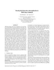
Quantifying the Impact <strong>of</strong> <strong>An</strong>omaly Detectors<br />
Consider a simple example where we have a system with an onboard sensor / anomaly detection algorithm<br />
that detects failures in advance with some probability <strong>of</strong> detection (PoD). If failure indications are detected<br />
early on, associated risks, downtime durations & failure costs are typically much lower<br />
Simulation-based trade studies can be used to optimize the sensor suite (PoD, false alarm rate, time to<br />
detect, etc) with the asset being monitored. This significantly improves reliability, reduces outage durations<br />
and reduces overall system operational risk.<br />
250<br />
200<br />
150<br />
100<br />
50<br />
0<br />
Failure<br />
System OK<br />
Downtime Duration Histogram, PoD = 50%<br />
(from 5000 Monte Carlo trials)<br />
Downtime Histogram<br />
PoD = 0%<br />
Detected,<br />
“Planned”<br />
Event<br />
Not detection<br />
“Unplanned”<br />
Event<br />
600<br />
500<br />
400<br />
300<br />
200<br />
100<br />
0<br />
Assumptions / Input<br />
Key Statistics<br />
Event Type Distribution Mean StDev<br />
Time to Failure (hr) Weibull 22181.6 9491.7<br />
Planned Downtime (hr) Lognormal 48 18<br />
Unplanned Downtime (hr) Lognormal 480 75<br />
Data & results for illustrative purposes only<br />
Downtime Duration Histogram, PoD = 50%<br />
(from 5000 Monte Carlo trials)<br />
Downtime Histogram<br />
PoD = 50%<br />
1200<br />
1000<br />
800<br />
600<br />
400<br />
200<br />
0<br />
Downtime Duration Histogram, PoD = 50%<br />
(from 5000 Monte Carlo trials)<br />
Downtime Histogram<br />
PoD =100%<br />
Downtime (hrs)<br />
Downtime (hrs)<br />
Downtime (hrs)<br />
(c) General Electric Company - 2010<br />
12
Unreliability, F(t)<br />
Beta<br />
Case Study 1 : From Weibull‟s to Loss Models<br />
• We show how life data analysis can be combined with a <strong>PHM</strong> metric (E.g. Probability <strong>of</strong><br />
Detection) to estimate a distribution <strong>of</strong> losses (costs)<br />
• Impact <strong>of</strong> model parameter uncertainty on “tail” risks .. Concept <strong>of</strong> VaR, TVaR, etc.<br />
Step 1 : Collect failure (“F”) &<br />
suspensions / right-censored “S” data<br />
Type<br />
Failure<br />
Time Type<br />
Failure<br />
Time<br />
S 0.824 F 4.900<br />
S 1.046 S 4.999<br />
S 1.416 F 5.271<br />
F 1.428 F 5.760<br />
S 1.801 F 5.772<br />
S 2.091 F 5.896<br />
S 2.419 F 6.093<br />
F 2.835 S 6.201<br />
S 2.905 F 6.242<br />
F 3.038 S 6.271<br />
S 3.182 F 7.495<br />
S 3.188 S 7.495<br />
F 3.394 F 8.282<br />
F 3.602 F 8.527<br />
F 3.607 F 9.181<br />
F 3.635 F 9.349<br />
F 3.670 F 9.379<br />
F 3.689 F 10.142<br />
F 4.441 F 11.303<br />
F 4.523 F 15.904<br />
99.00<br />
90.00<br />
50.00<br />
10.00<br />
Note: This example is for illustrative purposes only<br />
(c) General Electric Company - 2010<br />
5.00<br />
1.00<br />
Step 2 : Fit a standard survival model (E.g. Weibull)<br />
and estimate parameter uncertainties<br />
Probability - Weibull<br />
1.00 10.00<br />
100.00<br />
Time, (t)<br />
3.40<br />
2.92<br />
2.44<br />
1.96<br />
1.48<br />
1.00<br />
Value<br />
W2 MLE - SRM MED<br />
F=27 / S=13<br />
CB[FM]@95.00%<br />
2-Sided-B [T1]<br />
Sameer Vittal<br />
General Electric - Energy<br />
10/6/2010 13:32<br />
Lower<br />
95% CI<br />
5.00 6.00 7.00 8.00 9.00 10.00<br />
Eta<br />
Upper<br />
95% CI<br />
Eta = Weibull 7.5693 6.3807 8.9793<br />
Data 1<br />
Beta = 2.2462 1.7248 2.9252<br />
Var-Eta Var-Beta<br />
0.4352 Contour 0.0366 Plot<br />
0.0366 0.0916<br />
Weibull<br />
Data 1<br />
W2 MLE - SRM MED<br />
F=27 / S=13<br />
: 95%<br />
: 90%<br />
: 85%<br />
Sameer Vittal<br />
General Electric - Energy<br />
10/6/2010 13:33<br />
13
Case Study 1 : From Weibull‟s to Loss Models<br />
Step 3 : A simple simulation<br />
model in Excel (for demo<br />
purpose only )<br />
• Simple portfolio <strong>of</strong> 5 units ..<br />
• All have identical Weibull life<br />
distributions (same eta/beta)<br />
• No parameter uncertainty<br />
• Probability <strong>of</strong> Detection<br />
assumed to be 65%<br />
• If event is detected, lower<br />
costs …if missed,<br />
substantially higher cost<br />
distributions<br />
• Costs distributions (detected,<br />
missed) are lognormal<br />
• 20-Yr warranty assumed<br />
• Run Monte Carlo trials .. use<br />
any tool / VBA script<br />
Unit 1 Unit 2 Unit 3 Unit 4 Unit 5 Cost/Event Detect Miss<br />
Eta (yr) 7.57 7.57 7.57 7.57 7.57 Dist LOGN LOGN<br />
Beta 2.25 2.25 2.25 2.25 2.25 Mean $ 2,500 $ 25,000<br />
Simulated Failure Time (Yrs) StDev $ 1,000 $ 10,000<br />
TTF 1 8.7 4.9 5.7 9.5 4.4 CoV 0.4 0.4<br />
TTF 2 12.4 13.4 11.1 11.9 15.9 Mu 7.244 9.547<br />
TTF 3 18.5 19.7 16.9 20.8 22.5 Sigma 1.077 1.077<br />
TTF 4 26.7 20.4 20.3 27.7 28.2<br />
TTF 5 44.2 36.5 27.0 32.3 34.0 PoD 65% Avg-STD $ 1,576<br />
Table that tracks events<br />
Year Unit 1 Unit 2 Unit 3 Unit 4 Unit 5 Year Unit 1 Unit 2 Unit 3 Unit 4 Unit 5<br />
1 0 0 0 0 0 1<br />
2 0 0 0 0 0 2<br />
3 0 0 0 0 0 3<br />
4 0 0 0 0 0 4<br />
5 0 detect 0 0 miss 5 $ 2,629<br />
$ 25,543<br />
6 0 0 miss 0 0 6 $ 878<br />
7 0 0 0 0 0 7<br />
8 0 0 0 0 0 8<br />
9 detect 0 0 0 0 9 $ 1,630<br />
10 0 0 0 detect 0 10 $ 10,489<br />
11 0 0 0 0 0 11<br />
12 0 0 detect miss 0 12 $ 242 $ 7,916<br />
13 detect 0 0 0 0 13 $ 1,164<br />
14 0 detect 0 0 0 14 $ 1,740<br />
15 0 0 0 0 0 15<br />
16 0 0 0 0 detect 16 $ 2,093<br />
17 0 0 miss 0 0 17 $ 31,682<br />
18 0 0 0 0 0 18<br />
19 detect 0 0 0 0 19 $ 1,753<br />
20 0 miss 0 0 0 20 $ 69,889<br />
TOTAL $ 4,547 $ 74,258 $ 32,802 $ 18,405 $ 27,636<br />
Screenshot <strong>of</strong> a typical MC trial<br />
Note: This example is for illustrative purposes only<br />
(c) General Electric Company - 2010<br />
$/Yr $ 227 $ 3,713 $ 1,640 $ 920 $ 1,382<br />
14
Case Study 1 : From Weibull‟s to Loss Models<br />
Step 4 : A simple simulation<br />
model in Excel (for demo<br />
purpose only )<br />
• Same portfolio <strong>of</strong> 5 units ..<br />
• Unit Weibull‟s are not the same<br />
• Eta/Beta pairs obtained from<br />
Weibull covariance matrix ..<br />
Assume they are bivariate<br />
normal<br />
• This scenario includes<br />
parameter uncertainty<br />
• Rest is same ..<br />
• Run Monte Carlo trials ..<br />
Unit 1 Unit 2 Unit 3 Unit 4 Unit 5 Cost/Event Detect Miss<br />
Eta (yr) 6.78 6.65 6.73 5.40 6.34 Dist LOGN LOGN<br />
Beta 2.42 2.15 2.12 2.25 1.62 Mean $ 2,500 $ 25,000<br />
Simulated Failure Time (Yrs) StDev $ 1,000 $ 10,000<br />
TTF 1 5.5 3.3 9.4 3.9 5.7 CoV 0.400 0.400<br />
TTF 2 8.5 11.5 15.7 6.2 13.5 Mu 7.244 9.547<br />
TTF 3 13.8 14.9 18.4 11.7 20.8 Sigma 1.077 1.077<br />
TTF 4 20.5 17.0 27.3 16.7 22.7<br />
TTF 5 26.6 21.8 32.4 19.1 27.3 PoD 65% Avg/Yr/Unit $ 1,282<br />
Table that tracks events<br />
Year Unit 1 Unit 2 Unit 3 Unit 4 Unit 5 Year Unit 1 Unit 2 Unit 3 Unit 4 Unit 5<br />
1 0 0 0 0 0 1<br />
2 0 0 0 0 0 2<br />
3 0 0 0 0 0 3<br />
4 0 miss 0 miss 0 4 $ 27,043<br />
$ 15,805<br />
5 0 0 0 0 0 5<br />
6 detect 0 0 0 detect 6 $ 4,966<br />
$ 2,280<br />
7 0 0 0 detect 0 7 $ 10,975<br />
8 0 0 0 0 0 8<br />
9 detect 0 0 0 0 9 $ 2,353<br />
10 0 0 miss 0 0 10 $ 5,934<br />
11 0 0 0 0 0 11<br />
12 0 detect 0 detect 0 12 $ 376<br />
$ 15,296<br />
13 0 0 0 0 0 13<br />
14 detect 0 0 0 detect 14 $ 620<br />
$ 2,817<br />
15 0 detect 0 0 0 15 $ 1,402<br />
16 0 0 detect 0 0 16 $ 7,075<br />
17 0 0 0 detect 0 17 $ 4,365<br />
18 0 miss 0 0 0 18 $ 22,257<br />
19 0 0 detect 0 0 19 $ 3,727<br />
20 0 0 0 detect 0 20 $ 950<br />
TOTAL $ 7,939 $ 51,078 $ 16,736 $ 47,391 $ 5,097<br />
Screenshot <strong>of</strong> a typical MC trial<br />
Note: This example is for illustrative purposes only<br />
(c) General Electric Company - 2010<br />
$/Yr $ 397 $ 2,554 $ 837 $ 2,370 $ 255<br />
15
Case Study 1 : From Weibull‟s to Loss Models<br />
Weibull with<br />
Parameter<br />
Uncertainty<br />
Weibull<br />
Parameters<br />
Only<br />
Statistic<br />
Trials 5000 5000<br />
Mean $1,451 $1,350<br />
Median $1,228 $1,139<br />
Std Deviation $983 $898<br />
Variance $967,219 $806,465<br />
Skewness 3.20 2.58<br />
Kurtosis 29.99 18.82<br />
CoV 0.6777 0.6653<br />
Minimum $110 $94<br />
Maximum $16,957 $12,962<br />
Range Width $16,847 $12,868<br />
Weibull with<br />
Parameter<br />
Uncertainty<br />
Weibull<br />
Parameters<br />
Only<br />
Percentiles<br />
P0 $110 $94<br />
P10 $554 $502<br />
P20 $735 $676<br />
P30 $886 $824<br />
P40 $1,052 $973<br />
P50 $1,228 $1,139<br />
P60 $1,429 $1,334<br />
P70 $1,658 $1,553<br />
P80 $1,998 $1,881<br />
P90 $2,604 $2,420<br />
P100 $16,957 $12,962<br />
Typical Metrics :<br />
Value At Risk (VaR)<br />
• Percentile <strong>of</strong> interest<br />
(P95/P99) from loss model<br />
• Depends on <strong>business</strong> risk<br />
appetite<br />
Conditional Tail Expectation<br />
(CTE) or TVaR<br />
Mean<br />
EC<br />
VaR95<br />
CTE<br />
• “Expected” value <strong>of</strong> losses in<br />
tail (usually beyond the VaR<br />
limit)<br />
Risk-Adjusted Return On<br />
Capital (RAROC)<br />
• RAROC = Expected Return<br />
VaR or EC<br />
• Multiple uses in risk mgmt.<br />
Note: This example is for illustrative purposes only<br />
(c) General Electric Company - 2010<br />
16
Case Study 1 : Observations<br />
• Actuarial Methods .. Frequency/Severity or Discrete Event Simulationbased<br />
… ARE applicable to engineering asset management<br />
• Uncertainty matters !! (We all know this in <strong>PHM</strong>) .. But very critical for<br />
risk as models get larger, more realistic .. Include economic variables,<br />
shocks .. plus a lot <strong>of</strong> things that are hard to measure !!<br />
• “Expected” values and “traditional” metrics .. RoI, NPV, IRR, are helpful,<br />
but not enough.. <strong>The</strong> tail risk alone can wipe out a badly designed<br />
contract / portfolio<br />
• Communicate the value <strong>of</strong> <strong>PHM</strong> using the vocabulary <strong>of</strong> financial risk<br />
management : VaR, CTE, RAROC, EC, etc. ..<br />
• This is an EXTREMELY SIMPLE “made-up” example .. real projects<br />
require both model & parameter uncertainties, asset correlations (E.g.<br />
Copulas), systemic risk .. Contagion risk .. Risk attractors / diversifiers ...<br />
beyond the scope <strong>of</strong> this presentation<br />
(c) General Electric Company - 2010<br />
17
Optimal Shell Thickness, in<br />
$-<br />
$5,000<br />
$10,000<br />
$15,000<br />
$20,000<br />
$25,000<br />
$30,000<br />
Loss Cumulative Density Function,<br />
F(S)<br />
$-<br />
$1,000<br />
$2,000<br />
$3,000<br />
$4,000<br />
$5,000<br />
$6,000<br />
$7,000<br />
$8,000<br />
$9,000<br />
$10,000<br />
$11,000<br />
$12,000<br />
$13,000<br />
$14,000<br />
$15,000<br />
$16,000<br />
$17,000<br />
$18,000<br />
$19,000<br />
$20,000<br />
$21,000<br />
$22,000<br />
$23,000<br />
$24,000<br />
$25,000<br />
Loss Probability Mass Function,<br />
f(S)<br />
Failure Probability, %<br />
Failure Probability, %<br />
1<br />
2<br />
3<br />
4<br />
5<br />
6<br />
7<br />
8<br />
9<br />
10<br />
11<br />
12<br />
13<br />
14<br />
15<br />
16<br />
17<br />
18<br />
19<br />
20<br />
21<br />
22<br />
23<br />
24<br />
25<br />
0<br />
1<br />
2<br />
3<br />
4<br />
5<br />
6<br />
7<br />
8<br />
9<br />
10<br />
11<br />
12<br />
13<br />
14<br />
15<br />
16<br />
17<br />
18<br />
19<br />
20<br />
Case Study 2 : Probabilistic Design & <strong>PHM</strong><br />
Time-based FORM,<br />
SORM, MF-FOSM, etc<br />
Equivalent Weibull<br />
Pressure Vessel - Time Dependent Failure Probability<br />
Initial thickness = 0.38"<br />
100%<br />
90%<br />
Limit State 1<br />
80%<br />
Limit State 2<br />
System<br />
70%<br />
60%<br />
H A L<br />
A H<br />
Pressure Tank<br />
R<br />
2 Limit States (ASME)<br />
Design Variable : Shell Thickness<br />
50%<br />
40%<br />
30%<br />
20%<br />
10%<br />
0%<br />
Time, years<br />
Optimization<br />
Variation <strong>of</strong> optimal shell thickness<br />
with a warranty-based constraint<br />
Actuarial Loss Model<br />
Renewal Model<br />
Pressure Vessel - Expected Renewals<br />
Initial thickness = 0.38", warranty period is 25 years<br />
0.42<br />
100%<br />
14%<br />
2.5<br />
0.41<br />
0.40<br />
0.39<br />
0.38<br />
Fs(x) = 0.90<br />
Fs(x) = 0.80<br />
Fs(x) = 0.70<br />
Fs(x) = 0.60<br />
90%<br />
80%<br />
70%<br />
60%<br />
50%<br />
40%<br />
Loss PDF<br />
Loss CDF<br />
12%<br />
10%<br />
8%<br />
6%<br />
2.3<br />
2.0<br />
1.8<br />
1.5<br />
1.3<br />
Renewals<br />
0.37<br />
0.36<br />
0.35<br />
30%<br />
20%<br />
10%<br />
0%<br />
4%<br />
2%<br />
0%<br />
1.0<br />
0.8<br />
0.5<br />
0.3<br />
0.34<br />
Loss Amount, $<br />
Figure 10 : Actuarial Loss Model for a 25 year warranty, design shell thickness <strong>of</strong> 0.38"<br />
0.0<br />
Time, years<br />
Warranty loss amount, $<br />
Reference : Vittal S. & Phillips, R., “Modeling and Optimization <strong>of</strong> Extended Warranties<br />
Using Probabilistic Design”, RAMS2007, Orlando, FL (2007)<br />
(c) General Electric Company - 2010<br />
18
<strong>PHM</strong> As Part <strong>of</strong> Risk Management<br />
• <strong>PHM</strong> + Life-Extending Controls provide the “vital knobs” to manage operational<br />
risk in portfolio‟s <strong>of</strong> monitored assets<br />
• It‟s an “early warning system” .. For emerging/ systemic issues<br />
• Effective risk transfer mechanism .. From unplanned to planned maintenance<br />
(c) General Electric Company - 2010 19
Summary .. “Actuarial <strong>Engineering</strong>”<br />
<strong>An</strong> “engineering only” approach cannot unlock <strong>PHM</strong>‟s full value .. the<br />
associated financial service & <strong>business</strong> process is just as important<br />
“Actuarial Engineers” .. Engineers with skills in Operations Research,<br />
<strong>PHM</strong>, Reliability & Actuarial Science … are the people who can run the<br />
<strong>business</strong> <strong>of</strong> <strong>PHM</strong><br />
This field requires collaboration between the engineering and actuarial<br />
communities .. need to learn the other person‟s language ..<br />
Exciting area for research !!<br />
Thank You !<br />
(c) General Electric Company - 2010<br />
20